Meta-analysis and Meta-regression with R
Posted on Tue 13 October 2020 in R
Introduction
On December 2019, reports from severe acute respiratory syndrome in Wuhan, China, were linked to a novel coronavirus, now known as SARS-CoV-2, and the disease it causes was termed coronavirus disease 2019 (COVID-19).
The World Health Organization declared the COVID-19 outbreak a Public Health Emergency of International Concern on 30 January 2020, and a pandemic on 11 March 2020.
SARS-CoV-2 causes an interstitial and alveolar pneumonia, but in nearly 26% of patients it can lead to a severe disease, with multiple organ failure (references: 1, 2, 3, 4).
Thus, infection by SARS-CoV-2 can cause kidney injury, perhaps by direct impact of virulence, or via other renal insults such as volume depletion, hypoxia and cytokine storm. This has posed pressure to healthcare systems due to a shortage of dialysis staff, equipment and consumables throughout the world.
I recently co-authored an article regarding acute kidney injury (AKI) among patients infected with COVID-19 patients. The objective of the study was to systematically review the incidence of COVID-19-associated AKI, its related risks factors, need for renal replacement therapy (RRT) among patients with AKI and mortality according to current illness severity.
In this post I will show the code I used to meta-analyze the AKI incidence data among COVID-19 patients. As usual, the codes presented here are available on the corresponding folder on my GitHub portfolio.
Methods
Systematic Review methodology
My colleagues systematically searched PubMed, SCOPUS and Web of Science databases with the search terms “COVID-19” OR “SARS- CoV-2” OR “Coronavirus 2019” OR “2019- nCoV” AND “Acute Kidney Injury” OR “Kidney” OR “Nephrology” OR “Renal Disease” OR “Clinical Characteristics” OR “Clinical Features”.
Meta-analysis and meta-regression
The heterogeneity between studies sample sizes was expressed through I2 measure and τ2 statistic (estimated via maximum- likelihood). A Cochran”s Q test with k–1 df (in which k is the number of studies included) and with significance level α=0.10 (exclusively for this test) was conducted to assess if heterogeneity was significantly different from zero. If so, the heterogeneity was classified according to the observed I2 measure: ≤25%, between 25% and 50%, between 50% and 75% and between 75% and 100% were considered as low, moderate, high and very high heterogeneity, respectively. In case of significant heterogeneity, the meta-analyses were conducted assuming a random- effects model with the Hartung-Knapp adjustment (References: 6, 7).
The independent variables included in a multivariate meta-regression were: study location (China, Poland or the USA), study design (case series, prospective or retrospective cohorts), study setting (single or multicenter), AKI definition criteria, median age of patients in years, proportion of males patients in the sample size and proportion of patients with certain comorbidities, namely hypertension, other cardio-vascular diseases, diabetes, chronic pulmonary disease, chronic kidney disease (CKD) and cancer.
Results
Results of the systematic review
My colleagues found 21 studies and I was responsible for perform the meta-analysis. Overall, 15,536 patients with COVID-19 was the total sample size. Most studies (18) were from China, two were from the USA and one from Poland.
Incidence of AKI among patients with COVID-19
The meta-analysis showed an incidence of AKI associated with COVID-19 of 12.3% (95% CI=7.3% to 20.0%; Cochran’s Q=839.6 with 20 degrees of freedom, p<0.001; I2 = 97.6% and τ2 = 1.42).
Below I show the code that generated this result.
Loading packages
I used R software with RStudio in Windows 10 to perform the meta-analysis (the same steps can be followed in Unix systems). I opened a R session through RStudio, created a project, named it aki_demo and loaded all packages needed for the meta-analysis. The command to install them is:
# Run only once, if you do not have the packages installed yet
install.packages(c("meta", "here", "openxlsx"))
The packages and their dependencies will be downloaded from the internet and installed. After install, I must load them in the R session:
library(meta)
library(here)
library(openxlsx)
Load and inspect data
Now I can load the data. I prepared an Excel spreadsheet with an excerpt of the data of our paper and put inside a subfolder named data on my working directory. The current script I saved on a folder named src (for “source”). My project folder now look like this:
.
├── data
│   └── aki_demo.xlsx
├── output
├── src
│   └── aki_demo.R
├── .Rhistory
└── aki_demo.RProj
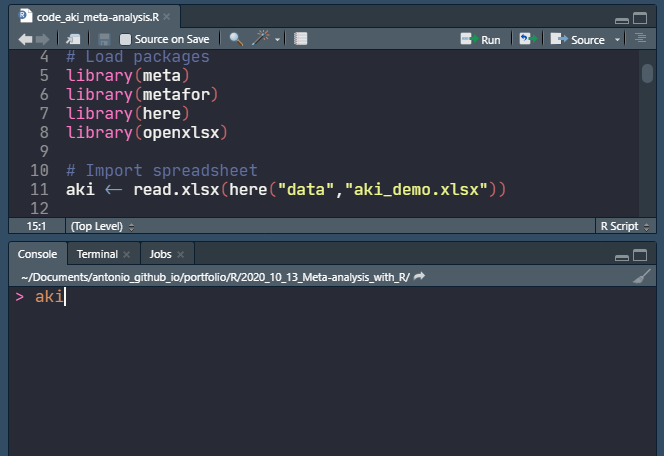
I load the spreadsheet into the R session memory with the command:
aki <- read.xlsx(here("data","aki_demo.xlsx"))
The <-, which is simply the “less than” < symbol followed by a dash symbol -, means “assigning”. I am assigning the data to the object named aki. The read.xlsx() function from openxlsx package reads the content of the spreadsheet and loads into a data frame, a tabular R format that holds data.
Note the usage of the here() function. here is a nice R package that helps file paths management. It ensures that my code will run smoothly on any computer, provided the directory structure is maintained. Thus, there is no need to hardcode file paths, improving code portability/reproducibility. The Dr. Jennifer Bryan’s post is a nice introduction to the here package.
To see the contents of the spreadsheet, type aki in the RStudio console window (bottom left area of RStudio window) and press Enter/Return or select the or put the cursor at the start of the line in the script window (top left) and press CTRL + Enter (⌘ Command + Enter on MacOS).
The first five columns of the output are below (I manually omitted the remaining of the table):
> aki
                          authors location sample_size control_aki case_aki
1           Tao Chen et al., 2020    China         274         245       29
2            W. Guan et al., 2020    China        1099        1093        6
3        Xiaobo Yang et al., 2020    China          52          37       15
4           Fei Zhou et al., 2020    China         191         163       28
5        Yingzhen Du et al., 2020    China          85          37       48
6      Chaolin Huang et al., 2020    China          41          38        3
7       Qingxian Cai et al., 2020    China         298         281       17
8       Yichun Cheng et al., 2020    China         701         665       36
9       Shaoqing Lei et al., 2020    China          34          32        2
10        Dawei Wang et al., 2020    China         138         133        5
11         Lang Wang et al., 2020    China         339         312       27
12   Jamie S. Hirsch et al., 2020      USA        5449        3456     1993
13      Blazej Nowak et al., 2020   Poland         169         152       17
14          Yi Zheng et al., 2020    China          34          27        7
15         Dawei Wang et al.,2020    China         107          93       14
16           Yuan Yu et al., 2020    China         226         169       57
17 Safiya Richardson et al., 2020      USA        5700        4330     1370
18    Guangchang Pei et al., 2020    China         333         298       35
19         Yanlei Li et al., 2020    China          54          25       29
20      Qingchun Yao et al., 2020    China         108          92       16
21     Chengfeng Qiu et al., 2020    China         104         102        2
Check that are 21 studies (rows) and the first five columns are: authors, location, sample_size (the number of COVID-19 patients), control_aki (the number of COVID-19 patients without AKI) and case_aki (the number of AKI cases among the COVID-19 patients).
To check the name of the other columns, type:
names(aki)

# Output:
 [1] "authors"        "location"       "sample_size"    "control_aki"
 [5] "case_aki"       "age"            "design"         "setting"
 [9] "aki_criteria"   "males_p"        "hypertension_p" "all_cardio_p"
[13] "diabetes_p"     "copd_p"         "ckd_p"          "cancer_p"
Then, it is possible to see that there are 16 columns in total. The bracketed number in the left side of the line is the index of the first element in the line (the count starts with [1] authors; the fourth element is [5] case_aki column, and so on).
To check the shape (dimensions) of the table I type:
dim(aki)

# Output:
[1] 21 16
The output tells that there are 21 rows and 16 columns indeed.
Calculating meta-analysis and inspecting results
Now I will use the metaprop() function from meta package to calculate the pooled incidence (a proportion) of AKI among COVID-19 patients and assign the results to aki_incidence_meta object:
aki_incidence_meta <- metaprop(event = case_aki, # numerator
                   n = sample_size, # denominator
                   studlab = paste0(authors,", ", location), # makes label by joining authors and location
                   data = aki, # dataframe name
                   sm = "PLO", # pooling calculation method
                   predict = TRUE, # provides prediction confidence interval
                   hakn = TRUE, # Hartung-Knapp correction
                   comb.fixed = TRUE, # displays fixed-effect results
                   comb.random = TRUE, # displays random-effect results
                   level.comb = 0.95, # confidence interval
                   method.tau = "ML", # heterogeneity calculation method
                   method.bias = "linreg",
                   warn = TRUE
)
Note that I type the command in this “list” format to allow easier reading of the code, it is not mandatory. The event argument is the numerator (thus aki_case column) and n is the denominator (sample_size column). I summarized above what the principal arguments do. Check metaprop()‘s documentation page here for more details. The meta package has other functions to perform meta-analysis with other kind of data. Check the documentation here.
Retrieving a summary of the aki_incidence_meta object produces this output:
# Command
summary(aki_incidence_meta)

# Output:
Number of studies combined: k = 21

                     proportion           95%-CI
Fixed effect model       0.2801 [0.2724; 0.2879]
Random effects model     0.1227 [0.0725; 0.2003]
Prediction interval             [0.0107; 0.6451]

Quantifying heterogeneity:
 tau^2 = 1.4231 [0.8378; 3.3344]; tau = 1.1929 [0.9153; 1.8260];
 I^2 = 97.6% [97.1%; 98.1%]; H = 6.48 [5.83; 7.20]

Test of heterogeneity:
      Q d.f.  p-value
 839.62   20 < 0.0001

Details on meta-analytical method:
- Inverse variance method
- Maximum-likelihood estimator for tau^2
- Q-profile method for confidence interval of tau^2 and tau
- Hartung-Knapp adjustment for random effects model
- Logit transformation
Since there was high heterogeneity, I chose to interpret the results through a random-effects model, yielding the numbers I quoted above. Below the results are the heterogeneity reports, results of Cochran’s Q test statistic, degrees-of-freedom and p-value confirming that the heterogeneity is not negligible and a summary of statistical methods used in the meta-analysis.
If you want to save this output directly to file, you could use the sink() method:
sink(here("output", "aki_incidence.txt"))
summary(aki_incidence_meta)
sink()
It will save the raw output in text format in a file named aki_incidence.txt into the output folder.
Producing a Forest plot
Now I will generate a Forest plot with forest() function (also from meta package) to visually represent the meta-analysis results and save it to a TIFF file. The commands below open the TIFF graphical device, produce the plot and then closes the device:
# Open the image device
tiff(filename = here("output", "plots", "aki_incidence.tiff"),
     compression = "lzw",
     res = 300,
     width = 3050,
     height = 1750)

# Produce the plot
forest(aki_incidence_meta,
             xlim = c(0, 1), # set axis limits
             comb.fixed =  FALSE, # omit fixed-effect model results
             leftlabs = c("Study, Location", "AKI cases", "Sample size"), # set left-side column names
             rightlabs = c("AKI incidence", "95% CI", "Weight"), # set right-side column names
             pooled.events = TRUE,
             col.predict = "black")

# Close the device and save the plot
dev.off()
Check other R graphical devices commonly used to save plots as images here.
Calculating a meta-regression
To calculate the meta-analysis, I needed just the sample size and number of events. I can use the remaining variables in the data frame to calculate a meta-regression to assess if aggregate measures of patients characteristics would be associated with increased risk of AKI occurrence. Below is the command I used:
aki_incidence_metareg <- metareg(aki_incidence_meta, ~ design + setting + location + age + males_p + aki_criteria + hypertension_p + all_cardio_p + diabetes_p + copd_p + ckd_p + cancer_p)
I used the aki_incidence_meta meta-analysis object as input to the metareg function. After a comma, I write a tilde ~ and the list all covariates separated by plus signs +. In R notation, the tilde separates the dependent covariate from the independent variables. Remember they are all columns from the spreadsheet I imported in the beginning. I check the results using the summary() function:
summary(aki_incidence_metareg)

# Output:
Mixed-Effects Model (k = 21; tau^2 estimator: ML)

  logLik  deviance       AIC       BIC      AICc
-20.3487   62.5815   76.6975   95.4989  418.6975

tau^2 (estimated amount of residual heterogeneity):     0.2864 (SE = 0.1130)
tau (square root of estimated tau^2 value):             0.5352
I^2 (residual heterogeneity / unaccounted variability): 77.00%
H^2 (unaccounted variability / sampling variability):   4.35
R^2 (amount of heterogeneity accounted for):            79.88%

Test for Residual Heterogeneity:
QE(df = 4) = 90.3774, p-val < .0001

Test of Moderators (coefficients 2:17):
F(df1 = 16, df2 = 4) = 0.6824, p-val = 0.7411

Model Results:

                                     estimate       se     tval    pval      ci.lb     ci.ub
intrcpt                               -7.1298   7.4538  -0.9565  0.3930   -27.8250   13.5654
designprospective                      3.9234   4.6568   0.8425  0.4469    -9.0058   16.8527
designretrospective                    4.8177   4.3793   1.1001  0.3330    -7.3411   16.9764
settingsingle_center                  -0.0597   1.0959  -0.0544  0.9592    -3.1023    2.9830
locationPoland                        -0.7740   1.7608  -0.4396  0.6829    -5.6628    4.1147
locationUSA                            1.5444   2.4229   0.6374  0.5585    -5.1826    8.2714
age                                    0.1119   0.1032   1.0844  0.3392    -0.1747    0.3985
males_p                               -5.7066   8.9694  -0.6362  0.5592   -30.6097   19.1964
aki_criteriaKDIGO                     -3.4725   2.6281  -1.3213  0.2569   -10.7691    3.8242
aki_criteriaKDIGO Expanded Criteria   -5.6275   4.2522  -1.3235  0.2563   -17.4334    6.1783
aki_criteriaSerum creatinine (Scr)    -1.5829   3.9282  -0.4030  0.7076   -12.4894    9.3236
hypertension_p                       -12.7624  10.2703  -1.2426  0.2819   -41.2774   15.7526
all_cardio_p                         -12.5110  25.5305  -0.4900  0.6498   -83.3950   58.3729
diabetes_p                            29.8351  25.7688   1.1578  0.3114   -41.7105  101.3807
copd_p                                 7.8958  38.3726   0.2058  0.8470   -98.6438  114.4353
ckd_p                                 77.4441  78.1549   0.9909  0.3778  -139.5486  294.4367
cancer_p                              -5.5262  20.2780  -0.2725  0.7987   -61.8269   50.7746

---
Signif. codes:  0 ‘***’ 0.001 ‘**’ 0.01 ‘*’ 0.05 ‘.’ 0.1 ‘ ’ 1
The estimate column is the magnitude of the effect of the variable upon the dependent variable (AKI incidence among COVID-19 patients). The bigger this number, the higher is the influence. Positive numbers mean higher risk. Negative numbers mean less risk. However, we must check the tval and its corresponding pval (p-value) columns. The tval test assumes a null hypothesis that estimate = 0. Therefore if pval is less than a pre-specified level of confidence (say, 5%), we can assume the estimate is significantly different than zero. Thus, we would assume that the variable would have influence over the outcome.
However, as you can see in the output, no variables were associated with AKI incidence with statistical significance.
Conclusion
With this I conclude this demonstration. To summarize I:
- Demonstrated how to import data into a R session;
- Introduced the
metapackage, a widely-used R package to meta-analysis calculation; - Demonstrated the rationale, execution and interpretation of meta-regression.
Check my published paper to see the results from a complete analysis of the systematically-reviwed data here.
Subscribe to my RSS feed, Atom feed or Telegram channel to keep you updated whenever I post new content.
References
-
Acute Respiratory Distress Syndrome and Death in Patients With COVID-19 in Wuhan, China
-
High burden of acute kidney injury in COVID-19 pandemic: systematic review and meta-analysis
-
On tests of the overall treatment effect in meta‐analysis with normally distributed responses
-
A refined method for the meta‐analysis of controlled clinical trials with binary outcome