Analyzing scRNA-Seq data with XGBoost

Posted on Wed 10 April 2024 in R

Introduction

Breast cancer is one of the most important morbidity and mortality cases around the world. In 2022, 2.3 million women were diagnosed with breast cancer and about 670,000 died from the disease, according to the World Health Organization.

Traditional breast cancer treatment with chemotherapy may be complicated by inherent characteristics of the tumor. Some women develop inflammatory breast cancer, a type of tumor with a high risk of metastasis and resistance to drugs such as doxorubicin and paclitaxel (Stevens et al. 2023).

Usually, tumors are a heterogeneous collection of cells. Some cells may be treatment-susceptible whereas others may have full-blown resistance to drugs. Imagine that would be a way to tell the cells apart and perhaps predict a prognosis for the patient, or change treatment options. With single-cell RNA-Seq (scRNA-Seq) studies, we may be one step closer to this objective. With scRNA-Seq data, we may assess gene expression patterns and use this information to differentiate cell identity.

Therefore, I decided to experiment with XGBoost, a popular machine-learning model used in classification and regression problems. Since I am interested in the differences between susceptible and resistant tumor cells at the gene expression level, I am dealing with a classification problem. Thus, I will train an XGBoost model with previous data and test with independent data to see if it can correctly predict the identity of a single cell based on its transcriptome. To this end, I will use raw data publicly available at the Gene Expression Omnibus (GEO) Datasets portal:

Train data: GSE163836 series by Peluffo et al. (2023)
Test data: (part of) GSE131135 series by Shu et al. (2020)

As always, the code of this demo will be deposited into my portfolio.

Installing packages

Install the following packages into your R library with the src/install_packages.R file:

# src/install_packages.R
packages <-
  c(
#"here",
#"tidyverse",
#"glue",
#"reticulate",
#"R.utils",
#"Seurat"
  )

lapply(packages, function(pkg) {
  if (!pkg %in% rownames(installed.packages()))
#
#install.packages(pkg)

})

Code outline

The main.R file contains the outline of this demonstration. First. let’s import some packages:

library(here)
library(tidyverse)
library(glue)
library(Seurat)
library(reticulate)

Next, I will set the folder structure of this demo project:

# main.R
folders <-
  c("src", "input", "intermediate", "output", "output/xgboost", "output/plot")

lapply(folders, function(folder) {
  path <- do.call(here, as.list(folder))

  if (!dir.exists(path)) {
#dir.create(path, recursive = TRUE)
  }
})

The next lines are all the steps I executed:

# main.R
# Scripts ----
## Prepare train data ----
source(here("src", "prepare_train_data.R"))

## Prepare test data ----
source(here("src", "prepare_test_data.R"))

## Gene (features) refinement ----
final_gene_list <-
  tibble(id = rownames(test_counts_transformed_scaled)) %>%
  inner_join(test_gene_names_df, by = "id") %>%
  inner_join(tibble(index = train_gene_names), by = "index")

final_gene_list %>% select(index) %>% write_tsv(here("intermediate", "final_gene_list.tsv"))

# Run XGBoost on Python ----
source_python(here("src", "run_xgboost.py"))

# Make plots ----
source(here("src", "make_plots.R"))

First, I will explain how I prepared the datasets for training and testing.

Preparing the data

Train dataset

I saved the HTTPS URL containing the raw scRNA-Seq objects into an object named URL_TRAIN and passed it as the first argument of the base R function download.file(), while saving it into the input folder with a sensible name:

# src/prepare_train_data.R
# Download data from GSE163836 project (Peluffo et al. 2023) (train dataset)
URL_TRAIN <-
  "https://www.ncbi.nlm.nih.gov/geo/download/?acc=GSE163836&format=file&file=GSE163836%5FIBC%5Fsc10x%5Fraw%5Fcounts%2ERData%2Egz"

train_data_path <- here("input", "raw_count_matrix_train.RData.gz")

if (file.exists(train_data_path)) {
  load(train_data_path)
} else {
  download.file(URL_TRAIN, destfile = train_data_path)

  load(train_data_path)
}

Since the file is an RData file, I loaded it into the working environment. It contained two objects: rawCounts and rawCounts.grp produced by the Seurat package. Seuratis a package designed to process single-cell genomics data. I believe it is (fittingly) named after the French pointillist painter Georges Seurat.

The rawCounts object is a transcript count matrix, whereas the rawCounts.grp is a factor vector containing the cell culture name of each cell:

head(rawCounts)
# 6 x 17202 sparse Matrix of class "dgCMatrix"

levels(rawCounts.grp)
# [1] "FCIBC02"   "FCIBC02PR" "SUM149PR"

I utilized the rawCounts.grp object to create a simplified vector, in which paclitaxel-resistant cells (whose names had the “PR” suffix) would be represented by the integer 1, and paclitaxel-susceptible cells would be 0:

# src/prepare_train_data.R
# Prepare single-cell data labels (train dataset) ----
train_labels <-
  ifelse(str_detect(rawCounts.grp, "PR"),
#     1,
#     0)

Then, I converted the count matrix into a Seurat object named train_counts:

# src/prepare_train_data.R
train_counts <-
  CreateSeuratObject(counts = rawCounts,
#                 project = "GSE163836")

train_counts
# An object of class Seurat 
# 32738 features across 17202 samples within 1 assay 
# Active assay: RNA (32738 features, 0 variable features)
#  1 layer present: counts

Thus, we can see the training dataset contains the transcriptomic quantification of 32738 transcripts among 17202 breast cancer cells.

After this step, the matrix is now amenable to transformation and metadata storage. With the next lines, which are provided by the Seurat documentation, I will:

transform the transcript counts;
perform quality control based on the percentage of mitochondrial transcript contamination;
scale and standardize transcript counts;
perform dimensionality reduction through PCA and UMAP, keeping the 3,000 most informative genes;
assign cells to clusters.

# src/prepare_train_data.R
train_counts_transformed <- train_counts %>%
  PercentageFeatureSet(pattern = "^MT-", col.name = "percent.mt") %>%
  SCTransform(vars.to.regress = "percent.mt") %>%
  RunPCA() %>%
  FindNeighbors(dims = 1:30) %>%
  RunUMAP(dims = 1:30) %>%
  FindClusters()

train_counts_transformed
# An object of class Seurat 
# 51656 features across 17202 samples within 2 assays 
# Active assay: SCT (18918 features, 3000 variable features)
#  3 layers present: counts, data, scale.data
#  1 other assay present: RNA
#  2 dimensional reductions calculated: pca, umap

After a while, I can store the transformed and scale for further use:

# src/prepare_train_data.R
# Save scaled data for future use ----
train_counts_transformed_scaled <- train_counts_transformed[["SCT"]]$scale.data

train_gene_names <- rownames(train_counts_transformed_scaled)

train_counts_transformed_scaled %>% 
  as_tibble() %>% 
  mutate(index = train_gene_names) %>% 
  relocate(index) %>%
  write_tsv(here("intermediate", "train_counts_transformed_scaled.tsv.gz"))

I do the same with a data frame containing metadata:

# src/prepare_train_data.R
train_metadata = tibble(
  umi = names(as_tibble(train_counts_transformed_scaled)),
  original_label = rawCounts.grp,
  label = train_labels
)

train_metadata %>% write_tsv(here("intermediate", "train_metadata.tsv"))

head(train_metadata)
# A tibble: 6 x 3
#   umi                          original_label label
#   <chr>                        <chr>          <dbl>
# 1 sample_10_AAACCTGAGCCAACAG-1 FCIBC02            0
# 2 sample_10_AAACCTGAGTGCGATG-1 FCIBC02            0
# 3 sample_10_AAACCTGCATTACCTT-1 FCIBC02            0
# 4 sample_10_AAACCTGTCAAGATCC-1 FCIBC02            0
# 5 sample_10_AAACGGGCACAAGTAA-1 FCIBC02            0
# 6 sample_10_AAACGGGCATGGGAAC-1 FCIBC02            0

Now, I will perform similar steps with the test dataset.

Test dataset

The test dataset comes from an independent study that used the same cell lines contained in the experiments that generated the train datasets. The authors also saved their raw data within an RData file:

# src/prepare_test_data.R
# Download data from GSE131135 project (Shu et al. 2020) (test dataset) ----
URL_TEST <- "https://www.ncbi.nlm.nih.gov/geo/download/?acc=GSE131135&format=file&file=GSE131135%5FBRD4JQ1%5Fsc10x%5Fraw%5Fcounts%2ERData%2Egz"

test_data_path <- here("input", "raw_count_matrix_test.RData")

if (file.exists(test_data_path)) {
  load(test_data_path)
} else {
  download.file(URL_TEST, destfile = glue("{test_data_path}.gz"))

  R.utils::gunzip(glue("{test_data_path}.gz"))

  load(test_data_path)
}

In this case, the RData file contained three objects instead of two: rawCounts (the gene count matrix, similar to its training equivalent), rawCounts.grp (the cell identities, also similar to its training equivalent) and rawCounts.ann (a data frame containing gene symbol annotations):

head(rawCounts.ann)
#                              id        symbol
# ENSG00000243485 ENSG00000243485  RP11-34P13.3
# ENSG00000237613 ENSG00000237613       FAM138A
# ENSG00000186092 ENSG00000186092         OR4F5
# ENSG00000238009 ENSG00000238009  RP11-34P13.7
# ENSG00000239945 ENSG00000239945  RP11-34P13.8
# ENSG00000239906 ENSG00000239906 RP11-34P13.14

However, the authors used other cell lines in their study, so I had to keep the data regarding the SUM149 cell line only. Similarly to the train dataset experiment, the authors worked with parental (identified as “SUM149DMSO”) and paclitaxel-resistant cultures (“SUM149RDMSO”). I created a metadata dataset to keep track of this information and used it to subset the original count matrix (also named rawCounts)

# src/prepare_test_data.R
# Subset data to keep specific samples ----
test_counts <- CreateSeuratObject(counts = rawCounts,
#                              project = "GSE131135")

test_metadata_filtered <- tibble(
  umi = as.vector(names(test_counts$orig.ident)),
  original_label = rawCounts.grp
) %>%
  filter(original_label %in% c("SUM149DMSO", "SUM149RDMSO")) %>%
  mutate(label = ifelse(str_detect(original_label, "R"), 1, 0))

test_metadata_filtered %>% write_tsv(here("intermediate", "test_metadata_filtered.tsv"))

test_counts <- subset(test_counts, cells = test_metadata_filtered$umi)

test_counts
# An object of class Seurat 
# 33694 features across 1636 samples within 1 assay 
# Active assay: RNA (33694 features, 0 variable features)
#  1 layer present: counts

Then, I applied the same QC/transformation steps and saved the results:

# src/prepare_test_data.R
## Transform, normalize, and reduce dimensionality ----
### https://satijalab.org/seurat/articles/sctransform_vignette
test_counts_transformed <- test_counts %>%
  PercentageFeatureSet(pattern = "^MT-", col.name = "percent.mt") %>%
  SCTransform(vars.to.regress = "percent.mt") %>%
  RunPCA() %>%
  FindNeighbors(dims = 1:30) %>%
  RunUMAP(dims = 1:30) %>%
  FindClusters()

# Save scaled data for future use ----
test_counts_transformed_scaled <- test_counts_transformed[["SCT"]]$scale.data

test_gene_names <- rownames(test_counts_transformed_scaled)

test_gene_names_df <- as_tibble(rawCounts.ann) %>%
  rename("index" = "symbol")

test_counts_transformed_scaled %>% 
  as_tibble() %>% 
  mutate(id = test_gene_names) %>%
  left_join(test_gene_names_df, by = "id") %>%
  relocate(index) %>%
  select(-id) %>%
  write_tsv(here("intermediate", "test_counts_transformed_scaled.tsv.gz"))

test_counts_transformed
# An object of class Seurat 
# 48790 features across 1636 samples within 2 assays 
# Active assay: SCT (15096 features, 3000 variable features)
#  3 layers present: counts, data, scale.data
#  1 other assay present: RNA
#  2 dimensional reductions calculated: pca, umap

Refine features (gene) list

To guarantee that train and test datasets had the same features (genes), I created a data frame holding the intersection of gene names contained in the scaled matrices:

# main.R
## Gene (features) refinement ----
final_gene_list <-
  tibble(id = rownames(test_counts_transformed_scaled)) %>%
  inner_join(test_gene_names_df, by = "id") %>%
  inner_join(tibble(index = train_gene_names), by = "index")

final_gene_list %>% select(index) %>% write_tsv(here("intermediate", "final_gene_list.tsv"))

This step concluded the data preparation. I saved all XGBoost input files into the intermediate folder:

.
├── input/
│   ├── raw_count_matrix_test.RData
│   └── raw_count_matrix_train.RData.gz
├── intermediate/
│   ├── final_gene_list.tsv
│   ├── train_metadata.tsv
│   ├── train_counts_transformed_scaled.tsv.gz
│   ├── test_metadata_filtered.tsv
│   └── test_counts_transformed_scaled.tsv.gz
├── output/
├── src/
│   ├── install_packages.R
│   ├── make_plots.R
│   ├── prepare_test_data.R
│   ├── prepare_train_data.R
│   └── run_xgboost.py
└── main.R

Run XGBoost

Then, I proceeded to train and evaluate an XGBoost model. I used the Python API. You can run Python scripts from R sessions using the reticulate package, as I demonstrated before. Just remember to install the required Python modules via pip, and indicate any conda or virtualenv environments to reticulate with use_condaenv() or use_virtualenv() functions.

With reticulate all set, you can source Python scripts directly from R:

# main.R
# Run XGBoost on Python ----
source_python(here("src", "run_xgboost.py"))

Let me walk through the src/run_xgboost.py script. First, I import all the required modules:

import json
from pathlib import Path

import matplotlib.pyplot as plt
import pandas as pd
import shap
from hyperopt import STATUS_OK, fmin, hp, tpe
from hyperopt.pyll import scope
from sklearn.metrics import roc_auc_score
from xgboost import XGBClassifier, plot_importance

Next, with the help of pathlib, I set all file paths:

# src/run_xgboost.py
# %% Set up paths
ROOT_DIR = Path.cwd()
TRAIN_METADATA_PATH = ROOT_DIR / "intermediate/train_metadata.tsv"
TEST_METADATA_PATH = ROOT_DIR / "intermediate/test_metadata_filtered.tsv"
TRAIN_COUNT_MATRIX_PATH = (
#ROOT_DIR / "intermediate/train_counts_transformed_scaled.tsv.gz"
)
TEST_COUNT_MATRIX_PATH = ROOT_DIR / "intermediate/test_counts_transformed_scaled.tsv.gz"
FINAL_GENE_LIST_PATH = ROOT_DIR / "intermediate/final_gene_list.tsv"
XGBOOST_DIR = ROOT_DIR / "output" / "xgboost"

Load data

Then, I load the gene list data frame into a pandas.DataFrame and saved the gene list into a Python list:

# run_xgboost.py
# %% Import refined gene list
gene_list = pd.read_csv(FINAL_GENE_LIST_PATH, sep="\t")
gene_list = gene_list["index"].to_list()

Next, I imported train and test datasets into pandas.DataFrame, treating the first column (the gene name) as the index:

# run_xgboost.py
train_count_matrix = pd.read_csv(TRAIN_COUNT_MATRIX_PATH, sep="\t", index_col=0)

Then, I filtered rows using the gene index to include only the genes in the gene_list object:

# run_xgboost.py
train_count_matrix = train_count_matrix[train_count_matrix.index.isin(gene_list)]

Sorted the index lexicographically (so train and test datasets have the same columns in the same order):

# run_xgboost.py
train_count_matrix = train_count_matrix.sort_index()

Finally, I transpose the pandas.DataFrame, to convert the rows into columns and vice-versa, so the features (genes) become columns, and rows become data points (single-cells). I also load the metadata file:

# run_xgboost.py
test_count_matrix = test_count_matrix.transpose()

test_metadata = pd.read_csv(TEST_METADATA_PATH, sep="\t")

I perform the same steps with the test dataset:

# run_xgboost.py
# %% Import test dataset
test_count_matrix = pd.read_csv(TEST_COUNT_MATRIX_PATH, sep="\t", index_col=0)
test_count_matrix = test_count_matrix[test_count_matrix.index.isin(gene_list)]
test_count_matrix = test_count_matrix.sort_index()
test_count_matrix = test_count_matrix.transpose()

test_metadata = pd.read_csv(TEST_METADATA_PATH, sep="\t")s

I have everything in place for running XGBoost. The next step is to find which hyperparameter configuration would provide me with a model with the best performance possible.

Hyperparameter optimization

XGBoost is a rather complex machine learning model, with several hyperparameters. The predictions of any XGBoost model are influenced by its hyperparameters, so it is recommended to spend some time optimizing them before training. See Carlos Rodriguez’s post for a brief review of XGBoost’s hyperparameters.

There are a few ways to obtain optimized hyperparameters, such as grid search and random search. See Rith Pansanga’s post for a brief review of some techniques. Based on this post, I decided to try a Bayesian optimization algorithm. First, I define a Python dictionary object named space with all hyperparameters as keys. For some of the keys, I define a range of values (a lower and an upper bound) with the help of the hyperopt module:

# src/run_xgboost.py
# %% Hyperparameter space for Bayesian optimization. Based on Rith Pansangas' tutorial available at https://medium.com/@rithpansanga/optimizing-xgboost-a-guide-to-hyperparameter-tuning-77b6e48e289d
space = {
    "max_depth": scope.int(hp.quniform("max_depth", 3, 7, 1)),
    "min_child_weight": scope.int(hp.quniform("min_child_weight", 1, 10, 1)),
    "subsample": hp.uniform("subsample", 0.5, 1),
    "colsample_bytree": hp.uniform("colsample_bytree", 0.5, 1),
    "learning_rate": hp.loguniform("learning_rate", -5, -2),
    "gamma": hp.uniform("gamma", 0.5, 5),
    "objective": "binary:logistic",
    "n_estimators": 1000,
    "early_stopping_rounds": 50,
    "eval_metric": "auc",
}

Observe that scope.int() must be placed around parameters that must be integers. Next, I define a function for score minimization. Here I set one minus the area under the receiver operating characteristic curve ROC AUC (1 - ROC_AUC) as the objective so hyperopt could provide, in reality, the hyperparameters associated with the maximum ROC AUC. Note that any other suitable metric could be used here. The function was named objective() and its input is a dictionary of hyperparameter space:

# src/run_xgboost.py
def objective(params):
    xgb_model = XGBClassifier(**params)

    xgb_model.fit(
        train_count_matrix,
        train_metadata["label"],
        eval_set=[
            (train_count_matrix, train_metadata["label"]),
            (test_count_matrix, test_metadata["label"]),
        ],
    )

    y_pred = xgb_model.predict_proba(test_count_matrix)

    score = 1 - roc_auc_score(y_true=test_metadata["label"], y_score=y_pred[:, 1])

    return {"loss": score, "status": STATUS_OK}

Next, I pass the objective() function and the space dictionary as the inputs to the hyperopt‘s fmin() function. This function will then test several combinations of hyperparameters (up to max_evals iterations), and through Bayesian statistics, find an optimized set of hyperparameters based on how any combination improves the AUC score. The output is assigned to the best_params object, which is a simple Python dictionary. After fmin() finishes running, I save the best_params into a JSON file for backup:

# run_xgboost.py
# %% Perform Bayesian optimization
best_params = fmin(objective, space, algo=tpe.suggest, max_evals=100)

# %% Save best params dictonary as a JSON file
with open(str(XGBOOST_DIR / "best_params.json"), "w") as file:
    json.dump(best_params, file)

Here are the output/best_params.json file contents:

{
    "colsample_bytree": 0.7879636151039555,
    "gamma": 1.8549947746359572,
    "learning_rate": 0.009073051650774098,
    "max_depth": 7,
    "min_child_weight": 3,
    "subsample": 0.7536343387772634
}

Training and evaluating the model

I can finally train the model with the optimized hyperparameters. I repeat the model definition, this time passing the best_params dictionary and complementing with the constant arguments:

# src/run_xgboost.py
# %% Repeat model fit, this time with the best hyperparameters
xgb_model = XGBClassifier(
    **best_params, n_estimators=1000, early_stopping_rounds=50, eval_metric=["auc"]
)

After that, I run the fit() method, passing as inputs the count matrix and the train labels:

# src/run_xgboost.py
xgb_model.fit(
    train_count_matrix,
    train_metadata["label"],
    eval_set=[
        (train_count_matrix, train_metadata["label"]),
        (test_count_matrix, test_metadata["label"]),
    ],
)

After a while, the fitting process finishes, and then I can obtain the ROC AUC score of the model. First, I use the predict_proba() method to obtain the individual cell probabilities for paclitaxel resistance. Next, I compare the predicted probabilities of the test dataset with the true test labels, and then save the resulting value into a text file:

# src/run_xgboost.py
y_pred = xgb_model.predict_proba(test_count_matrix)

roc_auc = roc_auc_score(y_true=test_metadata["label"], y_score=y_pred[:, 1])

with open(XGBOOST_DIR / "roc_auc.txt", "w") as file:
    file.write(f"{str(roc_auc)}\n")

This is the resulting AUC score:

roc_auc
# 0.6949359307013692

It is not a perfect score, but I was not expecting much, since it is a demonstration, without much sophistication.

Interpreting the model outputs

With the model in my hands, I can then collect the features’ importance metrics to see which genes were most informative for the classification. I collected gain and weight metrics for all informative genes into a pandas.DataFrame and saved it as a TSV file:

# src/run_xgboost.py
# %% Collect importance metrics into a dataframe
feature_importance_df = (
    pd.DataFrame(
        [
            xgb_model.get_booster().get_score(importance_type="gain"),
            xgb_model.get_booster().get_fscore(),
        ],
        index=["gain", "weight"],
    )
    .transpose()
    .reset_index()
    .rename(columns={"index": "gene"})
    .sort_values("weight", ascending=False)
)

feature_importance_df.to_csv(
    XGBOOST_DIR / "feature_importance.tsv", sep="\t", index=False
)

I also saved the top 15 most important features (by weight) with the help of matplotlib:

# src/run_xgboost.py
# %% Save importance (weight metric) plot with top 15 genes
plot_importance(xgb_model, max_num_features=15)
plt.savefig(str(XGBOOST_DIR / "top15_feature_importance_weight.png"))

Top 15 features (weight metric)

I also used the module shap to create a beeswarm plot to display a quantification of how much the top features in a dataset impact the model output:

# src/run_xgboost.py
# %% Use shap to help interpretation of the model
explainer = shap.Explainer(xgb_model)
shap_values = explainer(train_count_matrix)

# %% Beeswarm plot
shap.plots.beeswarm(shap_values, show=False)
plt.tight_layout()
plt.savefig(str(XGBOOST_DIR / "beeswarm_plot.png"))

shap Beeswarm plot

Observing the two plots, it seems that the expression of TPT1, JUND, KRT81, and CYBA differ between parental and paclitaxel-resistant cells. Looking at the beeswarm plot, CYBA and KRT81 appear to be downregulated in parental cells, since low expression values have negative impacts on the model output, diminishing the probability of being tagged by the model as paclitaxel-resistant, whereas for JUND1 the opposite is true: the higher its expression, the higher the positive impact on the model output, contributing to higher probability of being tagged by the model as paclitaxel-resistant.

Just to be sure, I went back to the data stored on the Seurat object and created more plots to assess the expression behavior of those genes. First, I created two lists containing the cells’ unique molecular identifiers (UMI):

# src/make_plots.R
# Get list of cells according to identity ----
parental_cells <- train_metadata %>%
  filter(label == 0) %>%
  pull(umi)

ptx_resistant_cells <- train_metadata %>%
  filter(label == 1) %>%
  pull(umi)

Then, I used the two vectors to annotate the cells on the object, storing the identities in the metadata slot:

# src/make_plots.R
# Set cells identities ----
Idents(object = train_counts_transformed, cells = parental_cells) <- "Parental"
Idents(object = train_counts_transformed, cells = ptx_resistant_cells) <- "Paclitaxel-resistant"

Then, I loaded the top 15 genes:

# src/make_plots.R
# Retrieve top 15 genes by importance metric (weight) ----
importance_df <- read_tsv(here("output", "xgboost", "feature_importance.tsv"))

## The TSV is ordered by descending weight values, take the first 15 rows
top15 <- importance_df %>% slice(1:15) %>% pull(gene)

Finally, I could plot ridge plots and UMAP plots:

# src/make_plots.R
# Make ridge and UMAP feature plots ----
RidgePlot(train_counts_transformed, features = top15, ncol = 3)
ggsave(filename = here("output", "plot", "ridge_plot.png"), width = 45, height = 20)

FeaturePlot(train_counts_transformed, features = top15)
ggsave(filename = here("output", "plot", "feature_plot.png"), width = 45, height = 20)

Ridge plot:

Ridge plot, 15 top genes

UMAP feature plot:

Feature plot, 15 top genes

Observing the ridge and feature plots, it indeed seems that CYBA is lowly expressed by the parental cells, with some paclitaxel-resistant cells having higher expression. Regarding KRT81, some paclitaxel-resistant cells have low expression, but others have expression revolving around tens of thousands of copies (the expression scale is logarithmic). The shape of the expression distribution of JUND1 is similar between parental and paclitaxel-resistant cells, but in the resistant cells, the tail is heavier: more resistant cells have higher expression in comparison with their parental counterparts. In summary, I believe the XGBoost model indeed captured these nuances of the data.

Mitochondrial transcript percentage plot

It is possible to obtain a violin plot to examine the proportion of mitochondrial transcripts (remember that the percent.mt metadata column was created during the data preparation step):

# src/make_plots.R
# Plot mitochondrial transcripts percent violin plot ----
## Save the cells identities as metadata column
train_counts_transformed[["identity"]] <- Idents(object = train_counts_transformed)

VlnPlot(train_counts_transformed, features = "percent.mt", split.by = "identity")
ggsave(filename = here("output", "plot", "percent_mt_violin_plot.png"), width = 10, height = 10)

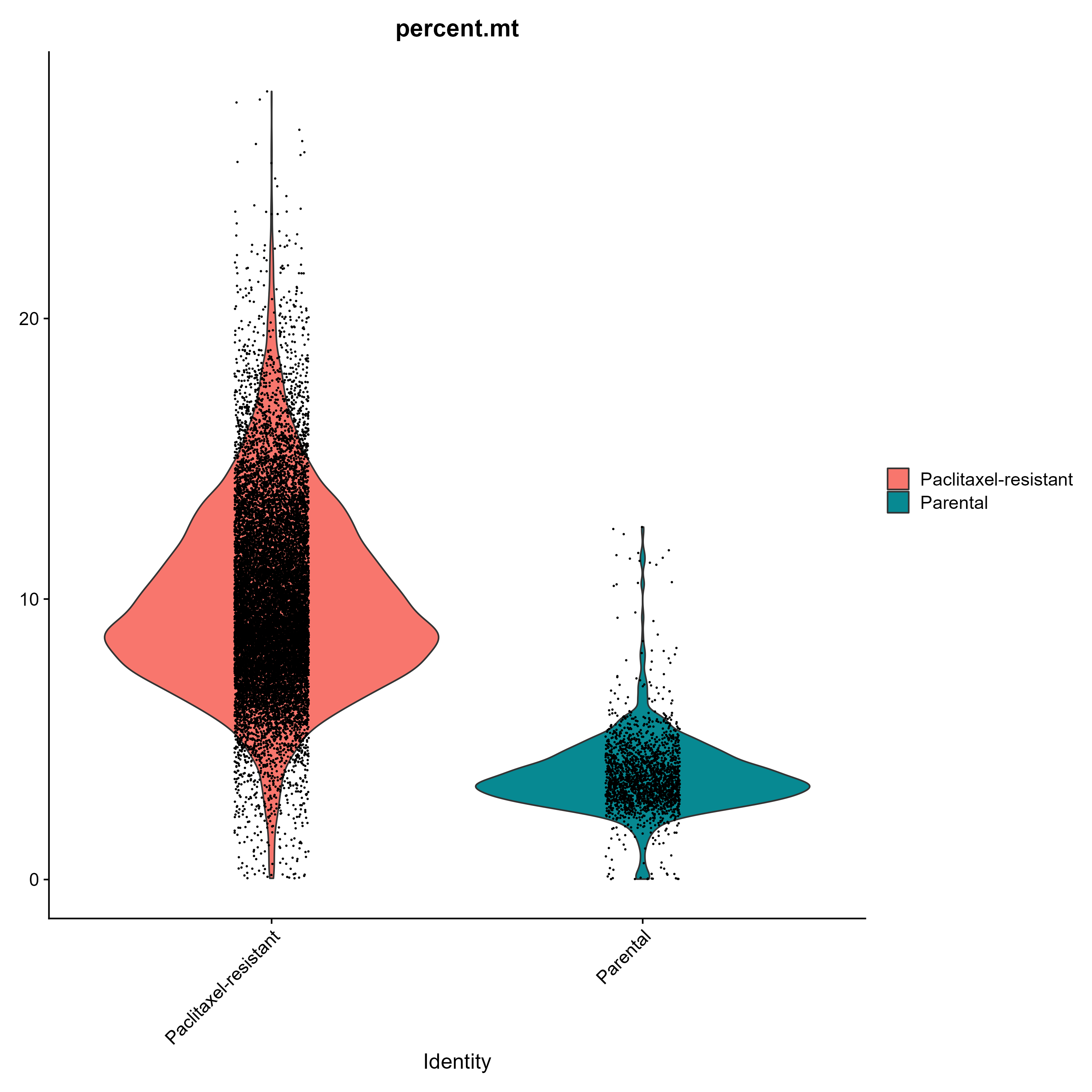
Proportion of mitochondrial transcripts.

For whatever reason, paclitaxel-resistant cells had higher levels of mitochondrial transcripts in comparison with parental cells. Further investigations can be performed to understand the reasons behind this difference.

Model backup

The trained model can be saved as a text file:

# src/run_xgboost.py
# %% Save model as text file
xgb_model.save_model(str(XGBOOST_DIR / "xgb_model.txt"))

Conclusion

In this post, I demonstrated:

A workflow to perform QC, transformation, standardization and dimensionality reduction of scRNA-Seq data with the Seurat R package;
How to perform Bayesian optimization of XGBoost hyperparameters;
Train and evaluate an XGBoost model;
Plots to help the model interpretation.

Subscribe to my RSS feed, Atom feed or Telegram channel to keep you updated whenever I post new content.