Differential Expression Analysis with edgeR in R

Posted on Mon 26 October 2020 in R

Introduction

In my previous post I demonstrated how to organize the CGC prostate cancer data to a format suited to differential expression analysis (DEA).

Nowadays, DEA usually arises from high-throughput sequencing of a collection (library) of RNA molecules expressed by single cells or tissue given their conditions upon collection and RNA extraction.

In terms of statistical analysis, DEA “means taking the normalized read count data and performing statistical analysis to discover quantitative changes in expression levels between experimental groups”. What are experimental groups? Consider for example, diseased versus healthy cells, treated cells versus non-treated cells (when someone is testing new drugs for example), and so on.

The edgeR package

There are some statistical packages in R that deal with DEA, such as edgeR, DESeq2 and limma. Here I will demonstrate a custom script to perform DEA with edgeR. The demonstration here is on Windows 10, but the same steps can be performed on Unix systems.

edgeR performs DEA for pre-defined genomic features, which can be genes, transcripts or exons, for example. In the present demonstration, we will quantify transcripts. Remember that genes can produce several transcripts through alternative splicing. The edgeR statistical model is based on negative binomial distribution. Prior to statistical analysis, edgeR normalizes gene/transcript expression counts via the Trimmed Mean of M-values (TMM) method. See Dr. Kevin Blighe’s comment in a Biostars forum topic for a brief discussion of edgeR and other DEA packages.

Without further ado, I will show how to set up a R session to run a DEA with edgeR, and how to interpret results. As usual, the code presented here is deposited on my portfolio at GitHub.

Install and load packages

First, I will install some new packages that I have not talked about. The first one is openxlsx, which is a package used to read/write Microsoft Office Excel spreadsheets. I will use it to conveniently save the output of the DEA.

The second is BiocManager. It is needed to install packages from Bioconductor project, which hosts Bioinformatics analysis packages that are not on the default R package repository.

The command below contains other packages I have used before, edit the comment if you already installed them:

# Run only once
install.packages(c("here", "tidyverse", "openxlsx", "BiocManager"))

Now I install edgeR and some more packages from Bioconductor. I will use them to annotate and convert the transcript/gene IDs to a gene symbol. Check their documentation: AnnotationDbi, annotate, org.Hs.eg.db, EnsDb.Hsapiens.v79 and ensembldb:

# Run only once
BiocManager::install(c("edgeR","AnnotationDbi", "annotate", "org.Hs.eg.db", "EnsDb.Hsapiens.v79","ensembldb"))

The :: is used when we wish to invoke the mentioned package directly (BiocManager in this case), without loading it into the memory.

Now, I will load just the here package to handle file paths for now, the rest will be loaded into R later.

library(here)

I will use the counts data frame I produced last time. Since I have saved it to my disk, I load it into the current R session. If you already have the counts data frame loaded in the session from the previous demonstration, this step is not necessary.

load(here("data", "counts.RData"))

Now I load the custom edgeR_setup() function I use to perform DEA with edgeR. I wrote the function in a R script with the same name and saved it on my src folder:

source(here("src", "edgeR_setup.R"))

Careful to not confuse the load() with source() functions. The former is used with R objects (*.RData) as input, whereas the latter takes a R script (*.R) as input and parses the commands contained in the script.

Check the edgeR_setup.R script. First, it loads the packages I installed before:

library(tidyverse)
library(openxlsx)

# Install trough BiocManager
library(edgeR)
library(annotate)
library(org.Hs.eg.db)
library(EnsDb.Hsapiens.v79)
library(ensembldb)
library(AnnotationDbi)

Now, check the function arguments:

edger_setup <- function(name, counts, replicates = TRUE, filter = TRUE, gene_id = c("NCBI", "ENSEMBL", "SYMBOL"), output_path) {

    # ... the function goes here ...
}

name: A string. An identifier for the experiment.
counts: The data frame containing the transcript counts.
replicates: A Boolean indicating if the samples are biological replicates. Defaults to TRUE.
filter: A Boolean indicating if lowly expressed transcripts should be filter out. Defaults to TRUE.
gene_id: A string indicating how transcripts are identified in the data frame. There are three options:
- NCBI: Entrez Gene Record ids
- ENSEMBL: ENSEMBL ids (ENS#)
- SYMBOL: Official HGNC gene symbol
output_path: A path and filename string where the results will be saved in Excel spreadsheet format. Example: "\some\path\results.xlsx".

The use of edgeR to analyze datasets with no biological replicates (replicates = FALSE) is discouraged. However, I prepared a special dataset of housekeeping genes based on the work by Eisenberg and Levanon (2013). I downloaded the HK_genes.txt supplementary file here and placed it in the data folder at my current work directory. I also wrote an auxiliary script named hk_genes.R and placed it in the src folder. Check below a representation of my current work directory, where main_dea_edgeR.R contains the commands of this demonstration.

.
├── data
│   ├── counts.RData
│   └── HK_genes.txt
├── output
├── src
│   ├── edgeR_setup.R
│   └── hk_genes.R
└── main_dea_edgeR.R

For now, I will use default values and indicate that the transcripts in the data frame are identified by ENSEMBL ids. Before running the function, I assign the output path string to the out_path object, which I include in the function call. Note that I gave the name prostate_cancer to identify the experiment, and it will also be the name of the sheet in the spreadsheet.

out_path <- here("output", "prostate_cancer.xlsx")

edger_setup("prostate_cancer", counts, replicates = TRUE, filter = TRUE, gene_id = "ENSEMBL", out_path)

The function will organize the data into groups based on the sample labels I applied previously (“case” and “control”), filter out genes with negligible expression and calculate the expression metrics, such as the logarithm of the fold-change (logFC) and counts per million transcripts (logCPM), as well as fit a statistical generalized linear model (GLM), calculating GLM coefficients (β) for each gene. The DEA then consists in perform a hypothesis test (quasi-likelihood F-test in this case), to test the null hypothesis that the coefficients are equal (or that β_control - β_case = 0). From the F-test statistics is then derived a p-value, which is adjusted by false discovery rate (FDR) to account for multiple comparisons.

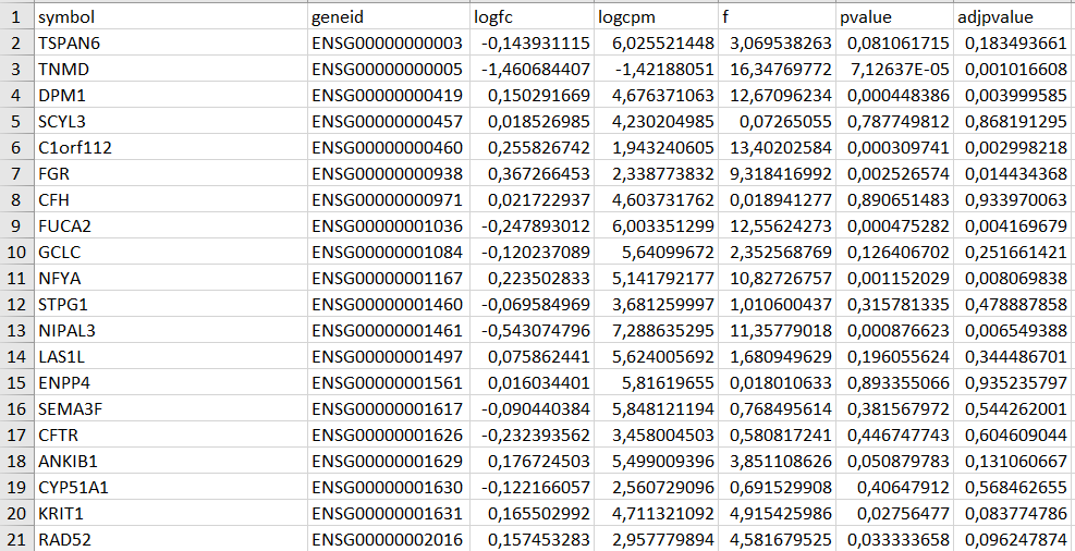
After a while, the function will generate a spreadsheet with the DEA results. See below an excerpt of the spreadsheet (with commas as decimal separators):

edgeR differential expression analysis in a prostate cancer dataset

Interpretation of the results

Note that there are seven columns:

symbol and geneid: transcript identifiers;
logfc: the base 2 logarithm of the fold-change (logFC), which is how much a quantity changes between two measurements — it is a ratio of two quantities. A logFC = 1 means that the expression of a certain gene was double in one condition than the other, a logFC = 2 means four-times higher expression, and so on. A logFC = -1 means half of the expression, a logFC = -2 means a quarter, and so on.
logcpm: the logarithm of the counts per million transcripts.
f: the quasi-likelihood F-test statistic.
pvalue and adjpvalue: the quasi-likelihood F-test statistic raw and FDR-adjusted p-values, respectively.

Note that the logfc column is the expression in cases group relative to control group. The edger_setup() custom function automatically organizes data to this end.

Usually, the researcher may want to further filter these results. For example, I like to consider not only the adjusted p-value, but also check which genes presented |logFC >= 1| (note the absolute value symbols here). Thus, if a gene passes these two criteria, I usually assume that it may have biological relevance for the disease/characteristic in study.

Conclusion

I demonstrated a custom function that uses edgeR package to perform differential expression analysis. Here is a summary of the requirements of the function:

A R data frame: rows are the transcripts, columns are the samples;
The samples must be labeled as “case” or “control” (in the column names);
The function outputs a spreadsheet with logFC and p-values;
The reported logFC are relative to the control group (control group is the reference);
The result spreadsheets can be filtered as the researcher wishes.

Subscribe to my RSS feed, Atom feed or Telegram channel to keep you updated whenever I post new content.