Parallelization with R
Posted on Mon 31 July 2023 in R
Introduction
Sometimes, some computations can be carried out in parallel. Certain large tasks can be divided into independent ones, allowing them to be solved at the same time, rather than waiting for each task to be solved sequentially.
I find the native R parallel functions such as mclapply(), or those from highly used packages such as snow to be cumbersome. Frankly, I assume I may never get those approaches to work.
This is why I got very happy when I recently discovered the furrr package. This package is from the tidyverse family, and as such, it is easy to use. With furrr, all the mental gymnastics I used to have when I tried parallelization in R is over.
The furrr package is the “marriage” between purrr and future packages. It has versions of the main mapping functions from purrr, but using future backend to execute computations in parallel and asynchronously.
In this post, I will demonstrate a simple way to achieve parallelization with R and furrr. The code of this demo is in my portfolio.
I will parallelize a series of differential expression analyses (DEA) of a dataset by Li et al. (2022). Check the Gene Expression Omnibus (GEO) summary page here. Briefly, they investigated the cellular alterations associated with the C9orf72 gene pathogenic repeat expansions. They performed single nucleus transcriptomics (snRNA-seq) in postmortem samples of motor and frontal cortices from amyotrophic lateral sclerosis (ALS) and frontotemporal dementia (FTD) donors as well as unaffected controls. They sampled three major brain cell populations (neurons, oligodendrocytes, and other glia) from both of the cortices.
Installing packages
Install the following packages into your R library with the src/installPackages.R file:
### src/installPackages.R ###
packages <-
  c(
    "here",
    "tidyverse",
    "glue",
    "openxlsx",
    "future",
    "future.callr",
    "devtools",
    "tictoc",
    "BiocManager"
  )

lapply(packages, function(pkg) {
  if (!pkg %in% rownames(installed.packages()))

    install.packages(pkg)

})

biocPackages <-
  c(
    "edgeR",
    "AnnotationDbi",
    "annotate",
    "org.Hs.eg.db",
    "EnsDb.Hsapiens.v79",
    "ensembldb"
    )

lapply(biocPackages, function(pkg) {
  if (!pkg %in% rownames(installed.packages()))

    BiocManager::install(pkg)

})
Now I create an outputs folder to hold the DEA results:
### main.R ###
# Paths ----
if (!dir.exists(here("outputs"))) { dir.create(here("outputs")) }
Next, I load all the functions I created for this demo:
### main.R ###
# Scripts ----
source(here("src", "functions.R"))
This script will load the following scripts in the functions folder: makeCountsDf.R, sourceFromGitHub.R, and runParallelDEA.R. I will explain each one at the appropriate moment.
Obtaining and preparing the data
The next step is executing the prepareData.R script:
### main.R ###
source(here("src", "prepareData.R"))
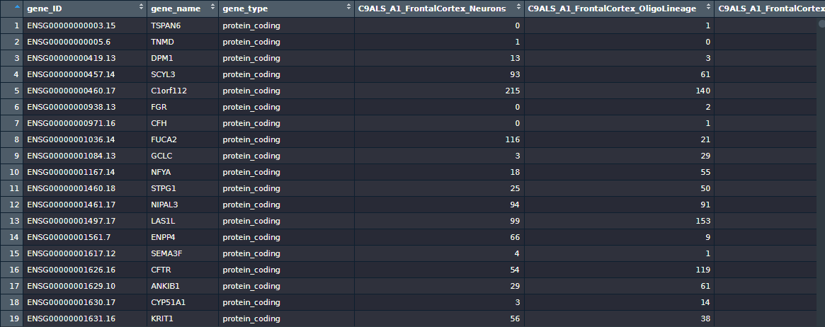
The script will start by loading the gene expression count data directly from the GEO FTP server into a data frame, and rounding up any number to the nearest integer just to be safe, since edgeR requires raw, integer counts:
### src/prepareData.R ###
# Load data ----
countDataOriginal <- read_tsv("https://ftp.ncbi.nlm.nih.gov/geo/series/GSE219nnn/GSE219278/suppl/GSE219278_allSamples_rsem_genes_results_counts_annotated.tsv.gz")

# Round up gene counts ----
countData <- countDataOriginal %>%
  mutate(across(where(is.numeric), ceiling))
This data frame has 60656 rows (genes/transcripts) and 117 columns. The first three columns are gene information: gene_ID, gene_name, and gene_type, leaving 114 columns to represent the samples (column indexes between 4 and 117).
Thankfully, the project authors gave very descriptive names to the columns, so I could identify right away their study design. I created a data frame named sampleInfo using the column names to extract information from each sample:
### src/prepareData.R ###
# Identify samples and outcomes ----
sampleInfo <- tibble(Names = names(countData)[4:length(names(countData))]) %>%
  separate(Names, into = c("outcome", "patientId", "location", "cellType")) %>%
  mutate(columnIndex = row_number() + 3)
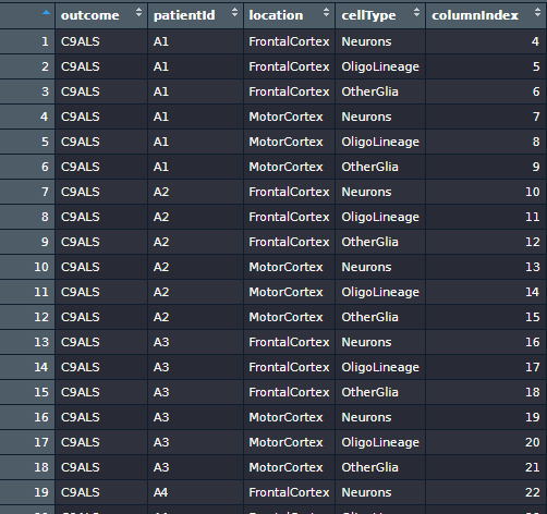
With the columnIndex column I created on the sampleInfo, I can extract the necessary cases/control combinations to generate 12 distinct data frames, by splitting the countData data frame.
By observing this table, I surmised they recruited three outcome groups: “C9ALS”, “C9FTD” and “Control”, with six, seven, and six individuals in each group, respectively. Since they collect three cell types from two cerebral cortices, we have six cortex/cell type combinations. Coupling with two distinct diseases, we can perform two case vs. control comparisons per combination. Therefore, we can perform \(3 \times 2 \times 2 = 12\) distinct DEAs.
To keep track of the samples in each of the 12 analyses, I created two lists of data frames, containing cases and controls, stratified by cortex and cell type:
### src/prepareData.R ###
alsDfsList <- sampleInfo %>%
  dplyr::filter(outcome == "C9ALS" | outcome == "Control") %>%
  group_by(location, cellType) %>%
  group_split()

ftdDfsList <- sampleInfo %>%
  dplyr::filter(outcome == "C9FTD" | outcome == "Control") %>%
  group_by(location, cellType) %>%
  group_split()
Next, I concatenate the two lists together:
### src/prepareData.R ###
allAnalysesList <- c(alsDfsList, ftdDfsList)
Finally, I can use the makeCountsDf() function to generate the 12 distinct gene count data frames. The function inputs are a data frame and a vector of column indexes, so it can convert the gene_ID into row names of the data frame and select the desired sample columns:
### src/functions/makeCountsDf.R ###
makeCountsDf <- function(dataFrame, columnIndexes) {

  counts <- dataFrame %>%
    dplyr::select(1, all_of(columnIndexes)) %>%
    rename_with(~ str_replace(.x, "C9ALS|C9FTD", "case")) %>%
    rename_with(~ str_replace(.x, "Control", "control")) %>%
    as.data.frame()

  row.names(counts) <- counts$gene_ID

  counts <- subset(counts, select = -c(gene_ID))

  return(counts)
}
I use a simple lapply loop to finally generate the countsDfsList object, which is a list of 12 data frames, each with the necessary samples for each distinct DEA as mentioned above.
### src/prepareData.R ###
# Split count data into 12 dataframes for differential expression analysis with edgeR ----
countsDfsList <- lapply(seq_along(allAnalysesList), function(index) {

  df <- allAnalysesList[[index]]

  cIdx <- df$columnIndex

  makeCountsDf(dataFrame = countData, columnIndexes = cIdx)

})
To keep track of each analysis, I named each element with a string contaning the disease, cortex and cell type by creating a string column combining the corresponding sampleInfo columns and pulling it to create a simple vector. With the vector, I set the countsDfsList element names:
### src/prepareData.R ###
allAnalysesNames <- sampleInfo %>%
  dplyr::filter(outcome != "Control") %>%
  dplyr::select(outcome, location, cellType) %>%
  distinct() %>%
  mutate(names = glue("{outcome}_{location}_{cellType}")) %>%
  pull(names)

names(countsDfsList) <- allAnalysesNames
In summary: I got the gene counts countData, and split it into 12 distinct data frames, stratifying by disease, cortex and cell type. Each one will allow a DEA with the edgeR package.
The runParallelDEA() function
By executing the sourceFromGitHub.R script, I sourced my edgeR_setup function directly from my GitHub portfolio:
### src/functions/sourceFromGitHub.R ###
URLs <- c("https://raw.githubusercontent.com/antoniocampos13/portfolio/master/R/2020_10_22_DEA_with_edgeR/src/edgeR_setup.R")

lapply(URLs, devtools::source_url)
In a previous post I demonstrated the edger_setup custom function that uses edgeR package to perform differential expression analysis.
Since I have 12 independent DEAs to perform, I surmised I could parallelize the computation, so I created the run function to demonstrate that sometimes parallel computation allows us to complete some tasks faster than if we executed them sequentially. Check the function code:
### src/functions/runParallelDEA.R ###
library(glue)
library(furrr)
library(future.callr)
library(tictoc)

runParallelDEA <- function(nWorkers) {

  plan(callr, gc = TRUE, workers = nWorkers)

  opts <- furrr_options(scheduling = TRUE, seed = TRUE)

  parallelFileNames <- glue("{names(countsDfsList)}_parallel_{nWorkers}_workers.xlsx")

  logMessage <- ifelse(nWorkers == 1, "Sequential execution", glue("Parallel execution with {nWorkers} workers"))

  tic(logMessage)
  future_walk2(
    .x = parallelFileNames,
    .y = countsDfsList,
    ~ edger_setup(
      name = as.character(which(parallelFileNames == .x)),
      counts = .y,
      gene_id = "ENSEMBL",
      output_path = here("outputs", .x)
    ),
    .options = opts
  )
  toc(log = TRUE)
  parallelTime <- unlist(tic.log(format = TRUE))
  tic.clearlog()

  parallelTime %>% write_lines(here("outputs", "tictoc_log.txt"), append = file.exists(here("outputs", "tictoc_log.txt")))

}
It is a convenient function around the execution of furrr‘s future_walk2 function based on the number of parallel workers (CPU cores). First, let me explain future_walk2: it applies a function (in this case, edger_setup) to each element of two vectors of the same length in parallel using the futures package backend. The number of simultaneous, parallel executions of edger_setup is controlled by the nWorkers parameter, which is passed over to the plan() function, which will use the future.callr API to finetune the futures package backend.
I chose future_walk2 because edger_setup does not return any value to the console; it just writes a spreadsheet with results directly to disk. Thus, I am interested in the “side-effect” of the function, which is exactly the purpose of walk-like functions.
edger_setup has three required inputs: name, counts and output_path. The counts parameter will receive each data frame stored in the countsDfsList list. With the parallelFileNames vector inside the function, I could satisfy both the name and output_path parameters.
In summary: the future_walk2 will map over two vectors (countsDfsList and parallelFileNames) and pass each element of both vectors simultaneously over to edger_setup.
Performing differential expression analysis (DEA) sequentially and in parallel
Now that I explained the logic behind the runParallelDEA() function, I can finally demonstrate how parallelization may accelerate the completion time of certain tasks. To this end, I created a numerical vector:
### main.R ###
# Run DEA  ----
nWorkers <- c(1, 2, 4, 6)

lapply(nWorkers, runParallelDEA)
Each number represents the number of workers (CPU cores) that I will loop over with lapply to pass over to runParallelDEA(). Six is the maximum number in the vector because my PC has this many cores.
Observe that the first element is 1: it will boil over to a sequential execution, since future_walk2 will use a single worker to process all 12 DEAs with edger_setup. The runParallelDEA() will count the number of seconds elapsed to complete all 12 DEAs and save it to the outputs/tictoc_log.txt file, displayed below:
### outputs/tictoc_log.txt ###
Sequential execution: 52.57 sec elapsed
Parallel execution with 2 workers: 35.78 sec elapsed
Parallel execution with 4 workers: 28.98 sec elapsed
Parallel execution with 6 workers: 26.89 sec elapsed
Notice how with six cores, the elapsed time to produce all 12 result spreadsheets is cut short by half! Now imagine the time gained in the calculation of more complex tasks, provided plenty of CPU cores and RAM size. Tasks that would run for several days or weeks if done sequentially can be performed in much shorter times if they are amenable to parallelization.
You can check the 12 spreadsheets and the tictoc log at the outputs folder (I included just only the set of spreadsheets produced by the 6 workers to avoid duplicate files on my GitHub portfolio).
Now that you know about the furrr package through my post, you can use it as a inspiration to try parallel computing with your use cases.
Conclusion
- I demonstrated the
furrrpackage for easy parallelization of tasks within R. - The
future.callrpackage finetunes thefuturebackend used byfurrr - Some tasks are completed quicker if they are amenable to parallelization
Subscribe to my RSS feed, Atom feed or Telegram channel to keep you updated whenever I post new content.