Training and Evaluating a Neural Network Model

Posted on Mon 22 April 2024 in Python

Introduction

In my previous post, I trained an XGBoost machine-learning model with single-cell RNA-Seq (scRNA-Seq) data to differentiate cell identity (parental cells versus paclitaxel-resistant cells) based on transcriptomic patterns.

As an exercise, I decided to use the same input data to experiment with other machine-learning models. In this post, I will demonstrate how I trained a neural network model with the PyTorch framework. PyTorch is a module designed for the development of deep learning using GPUs and CPUs in Python.

As usual, the code is available on my code portfolio at GitHub.

Code outline

The code for the demonstration is divided into two files: src/pytorch_nn_demo.py and main.py. The first contains classes, function definitions, and overall configurations, whereas the second contains the data import and actual execution of the code. If you would like to recap concepts about machine learning and neural networks before continuing, you may check the Appendix section.

Let’s start with src/pytorch_nn_demo.py.

`src/pytorch_nn_demo.py`

I recommend setting up a Python virtual environment. After you create the environment, install the required modules listed in the requirements.txt file. Install CUDA for your platform. I used version 12.4.1. I believe the code will work without CUDA, but I have not tested the code in this situation.

I start the script by importing all necessary modules:

# src/pytorch_nn_demo.py
# %% Python 3.10.4 | Pytorch 1.12.1 | CUDA 12.4.1
import copy
from collections.abc import Callable
from itertools import chain
from pathlib import Path
from typing import Type

import numpy as np
import torch
import torch.nn as nn
from sklearn.metrics import roc_auc_score
from torch.utils.data import DataLoader

Next, I set the computation device depending on the available hardware:

# src/pytorch_nn_demo.py
if torch.cuda.is_available():
    device = torch.device("cuda:0")
else:
    device = torch.device("cpu")

If a GPU is present and is compatible with CUDA, then all computations will be performed with it, and if not, the CPU will be used instead.

Next, I configured the neural network model, which I named NeuralNetwork, which inherits from a base module from PyTorch:

# src/pytorch_nn_demo.py
class NeuralNetwork(nn.Module):
    def __init__(
        self,
        n_features: int,
        n_neurons: int,
        n_output: int,
        activation_function: Callable[..., torch.FloatTensor],
        dropout: Callable[[torch.FloatTensor, float, bool, bool], torch.FloatTensor],
    ):
        super().__init__()
        self.dropout = nn.Dropout(dropout)
        self.n_features = n_features
        self.n_neurons = n_neurons
        self.n_output = n_output
        self.activation_function = activation_function
        self.layer1 = nn.Linear(n_features, n_neurons)
        self.layer2 = nn.Linear(n_neurons, n_neurons)
        self.layer3 = nn.Linear(n_neurons, n_output)
        self.sigmoid = nn.Sigmoid()
        self.double()

    def forward(self, input: torch.FloatTensor) -> torch.FloatTensor:
        fwd = self.activation_function(self.layer1(input))
        fwd = self.dropout(fwd)
        fwd = self.activation_function(self.layer2(fwd))
        fwd = self.dropout(fwd)
        fwd = self.sigmoid(self.layer3(fwd))
        return fwd

You can see that I defined two methods for the class: __init__() and forward(). The first serves to instantiate both the base module (see the super().__init__() snippet) and our modified module. The __init__() takes as arguments:

n_features: the number of independent variables (columns of the dataset matrix);
n_neurons: the desired number of neurons on the hidden layers;
n_output: the dimensionality the of output (dependent variable);
activation_function: one of several activation functions available in PyTorch;
dropout: a proportion of neurons to be randomly discarded in each layer independently.

The __init__() instantiates all given arguments as attributes of the class. Additionally, I instantiate:

a series of linear functions that will compose the layers of my model.
the sigmoid function: it takes the output of the last hidden layer (which is a matrix) and converts it to a vector/matrix of probabilities, depending on the number of output classes. For binary classification problems (which is my case), there are two classes: parental tumor cells and paclitaxel-resistant tumor cells. Then, the analysts can choose between soft and hard classification. In soft classification, you have a continuous distribution on the two classes (a vector with $S$ rows $\times$ 1 column with the probabilities, which is my case), whereas in hard classification the output is a matrix with $S$ rows $\times$ $C$ columns, where $S$ is the number of samples and $C$ the number of classes (2 or more).

The forward() method is responsible for performing the neural network forward pass calculations. See that it follows a specific order: the first two layers are my hidden layers, whereas the final one is my output layer. The first hidden layer takes the input and performs the linear combination of feature values and weights. The linear output is then handed over to the activation function, which is a non-linear function. The output of the first activation function is handed over to the second hidden layer, which performs the same steps, and, finally, the output layer takes the non-linear output of the second layer and converts it to a vector of probabilities with the help of the sigmoid function.

Notice the self.dropout(fwd) “sandwiched” between the layer’s calls. This indicates to the model that some of the weights set for each layer should be discarded. Since there are two dropout calls, they are performed on the weights of the first and second hidden layers. By the way, since my model contains two hidden layers, technically, we may call it a deep learning model.

Now, I will skip ahead to the core training/testing function I devised, the model_train_eval() function:

# src/pytorch_nn_demo.py
def model_train_eval(
    model: Type[NeuralNetwork],
    n_epochs: int,
    train_dataloader: Type[DataLoader],
    test_dataloader: Type[DataLoader],
    loss_function: Callable[..., float],
    optimizer: Callable[..., torch.FloatTensor],
    output_path: str,
    complementary_prob: bool = False,
) -> None:
    path = Path(output_path)

    if not path.exists():
        path.mkdir()

    best_roc_auc = -np.inf
    best_weights = None

    for epoch in range(n_epochs):
        train_loss, model_weights = train(
            model=model,
            train_dataloader=train_dataloader,
            loss_function=loss_function,
            optimizer=optimizer,
        )

        test_loss, roc_auc = test(
            model=model,
            model_weights=model_weights,
            test_dataloader=test_dataloader,
            loss_function=loss_function,
            complementary_prob=complementary_prob,
        )

        print(
            f"Epoch {epoch + 1}/{n_epochs}. Train loss: {train_loss}. Test loss: {test_loss}. ROC AUC: {roc_auc}"
        )

        if roc_auc > best_roc_auc:
            best_roc_auc = roc_auc
            best_weights = model_weights

            torch.save(best_weights, str(path / "best_weights.pth"))
            print(f"Current best epoch: {epoch + 1}")

This functions take as inputs:

our configured neural network/deep learning model;
the number of training/testing iterations (epochs);
two dataloaders: two objects for handling the datasets, one for training and another for testing dataset (more on that later);
the desired loss function;
the desired weight optimizer;
an output path to save the final model weights after finishing training;
a Boolean to indicate if complementary probabilities of the predictions should be used during testing (more on that later). Defaults to False.

The gist of this function is that, during the specified number of epochs, it will train the model, calculate the loss metric, and update the weights for each hidden layer. At the end of each epoch, it will then evaluate the current state of the model to assess the performance of the model, by producing predictions with the testing dataset and then comparing with the actual labels. Then, it will save the weights of the best model achieved at the desired output path. The model will print to standard output the current training and testing loss metrics, the current ROC AUC, and the epoch with the current best performance.

What happens during each epoch? In each epoch, the DataLoader object will take a subset, a batch, of samples from the dataset in use and perform the forward and backward pass calculations, as well as update the weights of each sample in the batch. In this way, models may be efficiently trained with large datasets without loading everything at once on memory. Thus, an epoch consists of a series of iterations on the dataset, until all computations are performed on all samples. In other words, an epoch is an iteration of iterations.

Now that I presented the overall function, I will then show the subfunctions: train() and test().

# src/pytorch_nn_demo.py
def train(
    model: Type[NeuralNetwork],
    train_dataloader: Type[DataLoader],
    loss_function: Callable[..., float],
    optimizer: Callable[..., torch.FloatTensor],
) -> tuple[float, torch.FloatTensor]:
    model.train()
    running_loss = 0.0
    for batch in train_dataloader:
        features, labels = batch
        features = features.to(device)
        labels = labels.to(device)
        optimizer.zero_grad()
        outputs = model(features)
        loss = loss_function(torch.squeeze(outputs), labels)
        loss.backward()
        optimizer.step()
        running_loss += loss.item() * labels.size(dim=0)

    train_loss = running_loss / len(train_dataloader.dataset)

    model_weights = copy.deepcopy(model.state_dict())

    return train_loss, model_weights

This train() function was inspired by Rob Mulla’s tutorial, with modifications. The function performs one round of training (one epoch), by taking one batch from the training dataset at a time and performing the forward pass calculations with our model definition (outputs = model(features)) and the loss metric calculation (by comparing the predictions with actual labels). PyTorch’s methods backward() and step() are responsible for automatically calculating optimized weights for all previous layers. The function then returns the loss metric and the current model weights and biases for one round of training. As you probably noticed, we simply had to configure the forward pass calculations, since PyTorch handles most of the more complicated calculations automatically.

Now let’s see the train() function:

# src/pytorch_nn_demo.py
def test(
    model: Type[NeuralNetwork],
    model_weights: torch.FloatTensor,
    test_dataloader: Type[DataLoader],
    loss_function: Callable[..., float],
    complementary_prob: bool = False,
) -> tuple[float, float]:

    model.load_state_dict(model_weights)

    model.eval()
    running_loss = 0.0
    labels_list = []
    predictions_list = []
    with torch.no_grad():
        for batch in test_dataloader:
            features, labels = batch
            labels_list.append(labels.tolist())
            features = features.to(device)
            labels = labels.to(device)
            outputs = model(features)

            y_preds = torch.squeeze(outputs)
            predictions_list.append(y_preds.tolist())

            loss = loss_function(torch.squeeze(outputs), labels)
            running_loss += loss.item() * labels.size(dim=0)

        test_loss = running_loss / len(test_dataloader.dataset)

    labels_flat = list(chain.from_iterable(labels_list))

    if complementary_prob:
        predictions_flat = [
            1 - el for el in list(chain.from_iterable(predictions_list))
        ]
    else:
        predictions_flat = list(chain.from_iterable(predictions_list))

    roc_auc = roc_auc_score(y_true=labels_flat, y_score=predictions_flat)

    return test_loss, roc_auc

The train function loads the weights and biases produced during the training round and loads them into the model class object. For each batch of the testing dataset, the function stores the actual labels and the predicted labels in two separate lists, labels_list and predictions_list, respectively. The predictions are generated by using the features of the batch as input for the model. The function then returns the loss metric of the model and the ROC AUC performance metric.

Thus, by chaining train() and test() into model_train_eval(), I can perform any number of epochs and keep track of how the model performs. Next, let’s put the code to work.

`main.py`

As usual, I start by importing all necessary modules, including the objects defined in src/pytorch_nn_demo.py:

# main.py
from itertools import chain
from pathlib import Path

import pandas as pd
import torch
import torch.nn as nn
import torch.optim as optim
from sklearn.metrics import roc_auc_score
from torch.utils.data import DataLoader
from torch.utils.data.dataset import TensorDataset

from src.pytorch_nn_demo import NeuralNetwork, device, model_train_eval

Next, I set up the file paths:

ROOT_DIR = Path.cwd()
TRAIN_METADATA_PATH = ROOT_DIR / "input/train_metadata.tsv"
TEST_METADATA_PATH = ROOT_DIR / "input/test_metadata_filtered.tsv"
TRAIN_COUNT_MATRIX_PATH = ROOT_DIR / "input/train_counts_transformed_scaled.tsv.gz"
TEST_COUNT_MATRIX_PATH = ROOT_DIR / "input/test_counts_transformed_scaled.tsv.gz"
FINAL_GENE_LIST_PATH = ROOT_DIR / "input/final_gene_list.tsv"
OUTPUT_DIR = ROOT_DIR / "output"

Remember that the input files come from my previous post. Therefore, I will re-use some code, with little modifications to load all dataset objects into pandas.DataFrame objects:

# main.py
# %% Import refined gene list
gene_list = pd.read_csv(FINAL_GENE_LIST_PATH, sep="\t")
gene_list = gene_list["index"].to_list()

# %% Import train dataset
train_count_matrix = pd.read_csv(TRAIN_COUNT_MATRIX_PATH, sep="\t", index_col=0)
train_count_matrix = train_count_matrix[train_count_matrix.index.isin(gene_list)]
train_count_matrix = train_count_matrix.sort_index()
train_count_matrix = train_count_matrix.transpose()

train_metadata = pd.read_csv(TRAIN_METADATA_PATH, sep="\t")
train_metadata["label"] = train_metadata["label"].astype(float)

# %% Import test dataset
test_count_matrix = pd.read_csv(TEST_COUNT_MATRIX_PATH, sep="\t", index_col=0)
test_count_matrix = test_count_matrix[test_count_matrix.index.isin(gene_list)]
test_count_matrix = test_count_matrix.sort_index()
test_count_matrix = test_count_matrix.transpose()

test_metadata = pd.read_csv(TEST_METADATA_PATH, sep="\t")
test_metadata["label"] = test_metadata["label"].astype(float)

Remember that the datasets have the samples (single breast tumor cells) as rows and features as columns (in this case, gene expression). Therefore, our trained neural network/deep learning model will differentiate (classify) between parental and paclitaxel-resistant cells.

To work with PyTorch, our data must be transformed into the torch tensor format. In my case, I will convert the two datasets into two TensorDataset objects:

train_tensor_dataset = TensorDataset(
    torch.tensor(train_count_matrix.values),
    torch.tensor(train_metadata["label"].values),
)

test_tensor_dataset = TensorDataset(
    torch.tensor(test_count_matrix.values),
    torch.tensor(test_metadata["label"].values),
)

Finally, I can generate two DataLoader objects so the datasets are amenable for batching during training and testing rounds:

# main.py
# %% Prepare datasets for batching
train_dataloader = DataLoader(train_tensor_dataset, batch_size=512, shuffle=True)

test_dataloader = DataLoader(test_tensor_dataset, batch_size=512, shuffle=False)

Notice that batch_size argument controls the size of the batch. Thus, I defined 512 observations per batch. Notice as well that the training dataset may be shuffled because it helps prevent the model from memorizing the order of the data. See Hengtao Tantai’s review and tips here. No shuffling is necessary on the testing dataset.

Next, I configured the neural network/deep learning model:

# main.py
# %% Configure neural network
n_features = train_count_matrix.shape[1]
n_output = 1
n_neurons = int((n_features + n_output) * (2 / 3))  # rule of thumb
dropout_rate = 0.2
activation_function = nn.ReLU()

model = NeuralNetwork(
    n_features=n_features,
    n_neurons=n_neurons,
    n_output=n_output,
    activation_function=activation_function,
    dropout=dropout_rate,
).to(device)

The datasets have 1253 features (gene expression columns) and have two classes: parental or paclitaxel-resistant, therefore, it can by represented by a single column of probabilities varying between 0 and 1. The higher the probability, the higher the chance that the tumor cells is paclitaxel-resistant.

There a few rules of thumb to determine the number of neurons in the hidden layers. See Sandhya Krishan’s post for a review. Here, I chose to use two thirds of the sum of inputs plus outputs ($(1253 + 1) \times 2/3 = 836$). I could have set different number of neurons for each layer, but to keep the model simple, they will have the same number of neurons.

I chose the rectified linear activation function or ReLU as the activation function of the hidden layers. Briefly, the ReLU is a non-linear function that returns the input as is only if its is higher than zero. Otherwise, if the input is zero or less, it will always return zero. See a brief review about ReLU here and why its characteristics are desirable during neural networks training.

Next, I defined the adaptive moment estimation algorithm (ADAM) with its default learning rateas the weights and bias optimizer, and the binary cross-entropy (BCE) as the loss function:

# main.py
# %% Run training/evaluation iterations
optimizer = optim.Adam(model.parameters(), lr=0.001)
loss_function = nn.BCELoss()

Finally, I can train/test the model for 250 epochs, and saving the best weights during all epochs into the output folder:

# main.py
model_train_eval(
    model=model,
    n_epochs=250,
    train_dataloader=train_dataloader,
    test_dataloader=test_dataloader,
    loss_function=loss_function,
    optimizer=optimizer,
    output_path="output"
)

While the training is occurring, summary of each epoch is printed to the standard output:

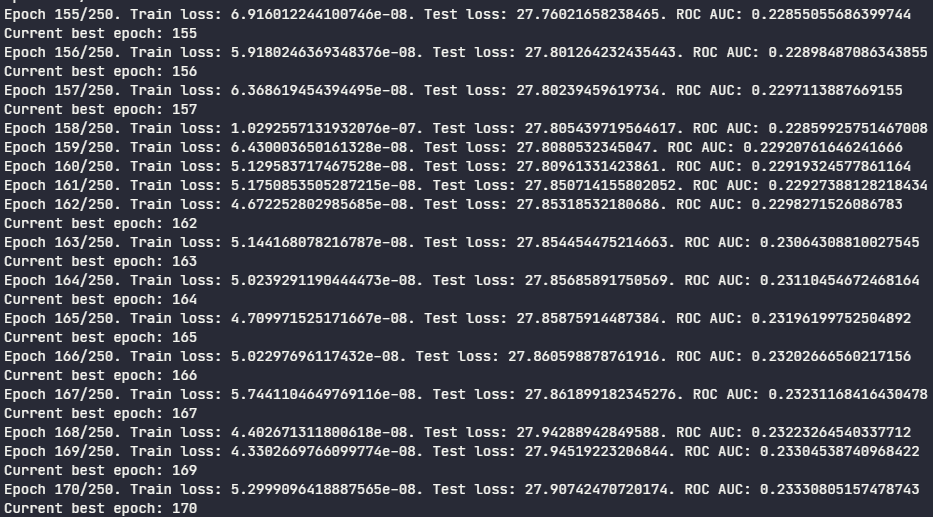
Printing epochs summary during training of the neural network model

As you may see on the image above, the ROC AUC was trending around 0.23 during the epochs. Since it is $<$ 0.50, the model is actualy a bad predictor for the positive class (paclitaxel-resistant cells). Apparently, it captured the patterns from parental cells better than the resistant ones. However, if we invert the model output by using their complementary probabilities, we can achieve ROC AUC $>$ 0.50:

main.py
# %% Check evaluation using complementary probabilities
model_train_eval(
    model=model,
    n_epochs=250,
    train_dataloader=train_dataloader,
    test_dataloader=test_dataloader,
    loss_function=loss_function,
    optimizer=optimizer,
    output_path="output",
    complementary_prob=True
)

During the new training, we see the AUC ROC score improved:

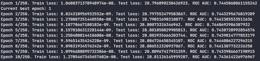
Printing epochs summary during training of the neural network model (complementary probability of the output)

As I mentioned above, the weights and biases of the best model were saved in the output folder. To load them into the model and perform predictions, follow the steps below:

# main.py
model = model
model.load_state_dict(torch.load("output/best_weights.pth"))
model.eval()

The model is now ready and loaded. Let’s evaluate the model. Obtain predictions by running the model with a feature matrix. For this example, I will use again the features from test dataset, after converting them to a PyTorch tensor:

# main.py
out = model(torch.tensor(test_count_matrix.values).to(device))

predictions_list = []

# %% Convert PyTorch Tensor to Python list
y_preds = torch.squeeze(out)
predictions_list.append(y_preds.tolist())

## Use Complementary probabilities (this step is specific for this demonstration only. Do not perform on your data, unless you know what you are doing)
predictions_flat = [1 - el for el in list(chain.from_iterable(predictions_list))]

# %% Calculate ROC AUC score
eval_roc_score = roc_auc_score(y_true=test_metadata["label"], y_score=predictions_flat)

eval_roc_score
# 0.7445068061155242

So I can see the final ROC AUC score converged to around 0.74. You may obtain a slightly different number due to the randomness introduced during shuffling of the drain dataset during epochs.

Conclusion

In this post I demonstrated how to configure a neural network/deep learning model through PyTorch, as well as how to configure a simple function to perform training and testing rounds of the model.

Subscribe to my RSS feed, Atom feed or Telegram channel to keep you updated whenever I post new content.

APPENDIX - Neural network and deep learning models: a brief recap

Machine-learning models, in general, aim to capture patterns in a dataset composed of features (independent variables) to predict the behavior of another variable, the output, dependent or status variable. Usually, we select a series of examples of labeled observations (samples) of those features (i.e. we know the status for each sample) and apply the desired model. This dataset is called the training dataset, and because of that, this rationale is called supervised learning. The objective of supervised learning is to obtain a statistical model capable of predicting the status of any other observation. We assess the model by applying the model to a test dataset, a completely separate collection of observations to ensure that the model works even with samples not previously encountered.

We assess the utility of the model during both phases: training and testing. During training, we compare the predictions of the model with the actual labels and calculate a loss (or cost) metric, which is a global metric that denotes how wrong was the model. Thus, all machine learning models strive to minimize this loss metric as much as possible during training. With neural networks/deep learning models, this is performed iteratively via a gradient descent algorithm.

Briefly, the gradient descent algorithm works by optimizing a series of weights, i.e., parameters (or coefficients) (usually represented by the symbols $\beta$ or $w$) for each observation. As a simple example, suppose that $y$ represents a probability and $\{x_1, x_2, x_3, ..., x_n\}$ represent the values of $n$ features. Therefore, the formula:

$$y = w_1 \times x_1 + w_1 \times x_2 + w_3 \times x_3 + ... + w_n \times x_n$$

relates the influence (hence the name weight) of each feature over the final probability. Thus, at each iteration, the model updates those weights based on the loss metric of the last iteration. Typically, we choose a number of iterations, or epochs, and assess at each epoch (or every few epochs, given a pre-specified interval), if the loss metric is satisfactorily decreasing. Neural network models also optimize biases, which are numeric constants that represent systematic errors in the data. The biases are added to each feature/weight multiplication product. For the sake of simplicity, I will not explore biases further, but keep in mind that whenever I mention weights, assume that biases are also involved.

How do neural networks derive those weights? We may conceptualize a neural network model as a series of sets of mathematical functions chained together, where the outputs of one set of functions are passed to the next set, and so on, until the last step, in which the loss metric is calculated (hence the name neural network, each set of functions are connected and share information in the same way that biological neurons do). Each set of functions is called a layer. Usually, each layer contains a linear combination (multiplication) of feature values times the weights. This combination is then handed over to a non-linear function, called the activation function. The activation function processes the input and hands it over to the next layer of the model. After the weights of all layers are computed (the forward pass computation), then we take the partial derivatives of the loss function with respect to all other operations (the backward pass computation). The result is a matrix of gradients, numerical values representing the influence of each weight on the final value of the loss function. Since the derivative of a function helps to find the minimum value of the original function, the model can update the starting weights for all layers in the next epoch, adjusting each weight in the direction that will minimize the loss metric, as mentioned above. Rinse and repeat until the pre-specified epochs end or the analyst is satisfied with the loss metric achieved.

The layers of a neural network are usually called:

Input layer: contains the feature matrix
Hidden layer(s): contain(s) neurons, activation functions work here. Each layer has its particular weight matrix.
Output layer: the loss metric calculation takes place here. The start of the backward pass takes place here. The weights for each previous layer are then updated.

The input layer is the “zeroeth” layer: it is represented by the feature values matrix, and no operations are performed here.

The hidden layers are the core of the model. All linear and activation functions are set at the hidden layers. They are called hidden layers because, usually, we do not check the numbers generated there, they are simply intermediate values for the output layer. The hidden layers operate by setting weight matrices with the dimensionality of the vector that represents each observation in the layer’s output. The number that represents this dimensionality is called the neurons. For example, imagine a neural network with one input layer, one hidden layer and one output layer. If we say that the input layer is a $S$ (samples) X $F$ (features) matrix, the output of the first hidden layer will have $N$ (neurons) X $F$ (features) dimensions. The number of neurons is pre-specified by the analyst. There are some rules of thumb for choosing the number of neurons in each layer, because too few neurons may result in suboptimal training, whereas too many neurons may cause overfitting of the model. The analyst may choose to apply neuron dropout rates. By pre-specifying a dropout rate (DR, in %), the analyst randomly discards the weights of DR% of the neurons at each layer independently (usually). Discard means the weights receive a value of zero. The neuron dropout is one of the most frequently used methods to reduce the risk of overfitting.

The output layer aggregates the computations from the previous layers and calculates the loss metric, which is used to update the weights. The weights are updated with the help of functions called optimizers, which use a learning rate to gauge how strongly the update in the value of the weights will be. A learning rate too small will result in a model taking longer to converge to a minimum value of the loss function, whereas a learning rate too large may find suboptimal results during training.

A neural network with two or more layers is called a deep learning model.

During testing, we assess performance metrics. Those metrics include, for example, accuracy, regression metrics, and the area under the receiver operating characteristic curve ROC AUC. We can even evaluate the model performance at each epoch (or every few epochs, given a pre-specified interval), in pace with the training procedure.

In summary, neural networks are nothing more than a series of linear matrix multiplication operations interspersed with non-linear operations. These procedural steps help capture linear and non-linear patterns in the data. The final result is a matrix of weights. The linear combination of feature values and weights (multiplication) captures all those patterns, helping predictions. We assess those predictions by using a separate dataset to evaluate if the model can correctly predict most of the previously known labels.