Working with Cancer Genomics Cloud datasets in a PostgreSQL database (Part 2)

Posted on Mon 12 October 2020 in SQL

Introduction

Recently I have been looking for publicly-available genomics datasets to test machine learning models in Python. During my searches for such a “toy dataset”, I came upon the Cancer Genomics Cloud (CGC) initiative.

Anyone can register in CGC and have access to open access massive public datasets, like The Cancer Genomics Atlas (TCGA). Most individual-level genomic data can only be accessed following approval of a Data Access Request through the Database of Genotypes and Phenotypes (dbGaP). For now, I guess the open data tier will suffice for this exercise.

This demonstration will be separated into two parts. In the first part I provided a brief run-down of how I queried the CGC to obtain genomic data from cancer patients and the first steps into preparing a local PostgreSQL relational database in my computer.

Here in the second part I will use a customized Python to help with the import of genomic data into the PostgreSQL database.

Why use Python to import the genomic data into the PostgreSQL database

In the first part of this demonstration I mentioned that I got more than 200 files containing the raw counts of gene expression in the prostate cancer individuals, each corresponding to a individual with prostate gland cancer. Unfortunately, the counts files do not have the patient identification. This information is only available in the files.tsv (and in my allfiles table in the database consequently), which indicates which count file belongs to each patient. Therefore, I must include the count file name alongside the gene counts.

Below I have an illustration of the problem. I have two files, count_A and count_B:

# count_A
ENSG00000000003.13 4000
ENSG00000000005.5 5
ENSG00000000419.11 1800

# count_B
ENSG00000000003.13 3000
ENSG00000000005.5 25
ENSG00000000419.11 500

In this state, I cannot know which patients provided the samples that generate count_A and count_B. But if I add a new column with the filename:

# count_A
ENSG00000000003.13 4000    count_A
ENSG00000000005.5 5   count_A
ENSG00000000419.11 1800    count_A

# count_B
ENSG00000000003.13 3000    count_B
ENSG00000000005.5 25  count_B
ENSG00000000419.11 500 count_B

I can now cross-reference with the allfiles table, and identify which file belong to each patient:

case_id file_name
case0001 count_A
case0002 count_B

Thus, I created a relation between the gene expression quantification and their patients of origin. Keep in mind that the gene counts file have thousands of rows, each corresponding to one human gene/alternate transcript. Therefore, I must:

Automate the creation of the third column containing the file name in all 200+ gene count files;
Join the modified files into a single, unified data frame;
Import the data frame into the tcga database.

With only programming language — Python — I can do all three requirements above. So that’s why I used Python: it is a very powerful, versatile language!

Create Python virtual environment

Follow instructions to install Python in Windows here. Ensure that Python is included in your Windows PATH. Python usually comes pre-installed in several Unix distros and already included in the PATH.

First, I will create a virtual environment to hold the necessary Python modules for my customized Python script. This is good practice — as I explained in my previous post different environments isolate programs for different uses, ensuring compatibility. In the post I talked about miniconda, but the principle is the same for Python here.

Otherwise, you can create a miniconda environment with Python included, and install all Python packages via miniconda channels. Since I will not use any other software besides Python here, there is no need to use miniconda, in my opinion. I created a virtual environment using Python’s virtualenv tool. Currently, I am using Python version 3.8.

In the TCGA folder I open a PowerShell and issue the commands below:

python -m pip install --user virtualenv

python -m venv venv

The first command installs the program virtualenv (venv) via the Python package manager pip. The second command uses venv to create a virtual environment deposited in a folder named venv in the current directory (TCGA folder in this example). You can also provide a complete path like this:

python -m venv C:\Users\some_path\TCGA\venv

Of course, you can call the virtual environment as you wish.

Activate the virtual environment

Still in the TCGA folder, I type the command:

venv\Scripts\activate

The virtual environment is ready to be used. I will install the necessary modules for the work.

Install Python modules into the virtual environment

The modules I will install are:

dask: to create the unified data frame with the gene expression;
psycopg2-binary and sqlalchemy: to connect with the PostgreSQL database and push the dataframe into it.

pip install "dask[complete]" psycopg2-binary sqlalchemy

The modules will be downloaded from the internet and installed at the venv folder. Additional dependencies, such as pandas (a widely-used data analysis and manipulation tool) and NumPy (package for scientific computing), used by dask, will be downloaded as well.

Creating Python credentials to access PostgreSQL database

To access the tcga database through Python, we need to configure credentials for the connection.

In the terminal I type:

psql -U postgres -d tcga -c "CREATE USER <USER_NAME> with encrypted password '<PASSWORD>'"

psql -U postgres -d tcga -c "GRANT ALL PRIVILEGES ON DATABASE tcga TO <USER_NAME>"

<USER_NAME> and <PASSWORD> are placeholders for my username and password, respectively, since it is good practice to NEVER share sensitive information.

Then, I created a file named settings.py and put it in a src folder with the following content:

DB_FLAVOR = "postgresql"
DB_PYTHON_LIBRARY = "psycopg2"
USER = "<USER_NAME>"
PASSWORD = "<PASSWORD>"
DB_HOST = "localhost"
PORT = "5432"
DB_NAME = "tcga"

Create one yourself with the user name and password you specified on the previous step. The other parameters can be left as they are. The 5432 port is usually the default port configured during installation to connection to PostgreSQL. Change it if needed, of course. localhost means that the PostgreSQL is running locally in my computer.

Then, to keep the organization of my folder, I added my tcga_processing_counts.py customized script to the src folder. The folder structure is now like this:

.
└── TCGA
    ├── data
    │   ├── counts
    │   │   └── [200+ *.counts.gz files]
    │   ├── focal_score_by_genes
    │   ├── fpkm
    │   ├── gene_level_copy_numbers
    │   ├── cases.tsv
    │   ├── demographic.tsv
    │   ├── files.tsv
    │   └── follow_up.tsv
    ├── src
    │   ├── settings.py
    │   └── tcga_processing_counts.py
    ├── main_tcga.ps1
    └── main_tcga.sh

Running the script

Back in the TCGA folder, I type in the PowerShell:

python src\tcga_processing_counts.py

This will start the script, which has eight steps:

Set up PostgreSQL connection object: psycopg2 and sqlalchemy modules use the credential of the settings.py;
Set up project paths: locate the data folders;
Decompress the .counts.gz files;
Make a list of all uncompressed files;
Create a function ready to return a pandas.DataFrame: this is when I add the third column with the filename in the counts files;
Create a list of commands to apply the read_and_label_csv function to all files;
Using dask‘s delayed method, assemble the pandas.DataFrames into a dask.DataFrame;
Send the dask.DataFrame to the database.

There is an optional step before step 8 to export the dask.DataFrame as HUGE CSV file that I disabled by default. WARNING: IT USES A LOT OF RAM AND CPU.

The use of dask for this job is crucial. pandas works by loading all data into the RAM. However, since there are several files of considerable size, it would overload my available RAM. dask is suited for larger-than-memory datasets, since it operates by lazy evaluation: it break operations into blocks and specifies task chains and execute them only on demand, saving computing resources.

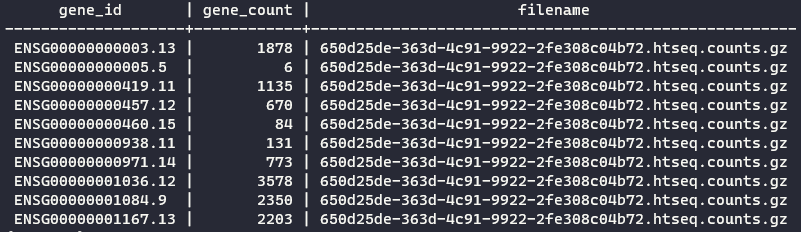
Go check the contents of my tcga_processing_counts.py in my portfolio. By default, it will create a table named gene_counts in the tcga database. See an excerpt of the final result:

Gene counts table in tcga database

Finishing touches

With the gene expression counts dataset imported in the database, it is time to create the filename (gene counts)/patient relation as I explained in the beginning of the post. In the terminal again, I type:

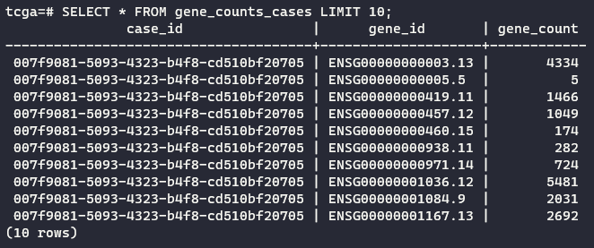
psql -U postgres -d tcga -c "CREATE TABLE gene_counts_cases AS SELECT DISTINCT case_id, gene_id, gene_count FROM gene_counts LEFT JOIN allfiles ON gene_counts.filename = allfiles.file_uuid WHERE gene_id LIKE '%ENSG%'"

The command above links the two tables by their information in common: the filename of the gene counts, which is named filename in the gene_counts table and file_uuid in allfiles table that we created before.

See an excerpt of the final result:

Gene counts table in tcga database: counts/patient relation

With this I conclude the second and last part of this demonstration. There is still missing the outcome information, which is located in the follow_up table in the database. However, the gene_counts_cases table is not yet ready to be linked. I need to pivot this table, but PostgreSQL has a limit of 1600 columns. Perhaps if I import this table into a session in R, it will be possible to transform the table. Additionally, I will perform differential expression analysis for sequence count data.

Conclusion of Part 2

In this part I:

Demonstrated how Python can be used to create data frames larger-than-memory with dask module;
Demonstrated how to connect Python to PostgreSQL databases with psycopg2 and sqlalchemy modules;
Demonstrated simple LEFT JOIN operation to link gene counts to individual cases of prostate cancer.

Go back to Part 1.