FASTQ to Annotation (Part 4)

Posted on Tue 06 October 2020 in Unix

Introduction

In a previous post, I showed how to configure an Ubuntu system to install Bioinformatics programs.

Now, using the environment I created, I will demonstrate a bash script, FastQ_to_Annotation.sh that takes next generation sequencing (NGS) raw reads from human whole genome sequencing as input and produces variant annotation as output. Variant annotation is the process of identifying genetic variants in some genomic DNA sample, and assess, for example, if any of the found variants have any effect on phenotype, such as increased susceptibility to certain diseases.

In the first part, I showed how to search for NGS projects deposited in National Center for Biotechnology Information (NCBI) databases from which I can download sequencing reads later to use with the script.

In the second part, I showed how to retrieve raw genome sequencing reads in the form of FASTQ files, which are deposited in SRA.

In the third part, I made the final preparations for the FastQ_to_Annotation.sh script demonstration using the FASTQ files obtained in the second part.

Here in the fourth and final part, I finally can summarize the inner workings of the FastQ_to_Annotation.sh script.

FastQ_to_Annotation.sh parameters

Activate your miniconda environment if needed and go to your demo folder. Make sure you have the FASTQ files and a refs folder with the human genome FASTA files and the other various supporting files.

The script needs 10 command line parameters to work correctly. They are:

Mate-pair FASTQ files name root (without extension) (absolute file path)
Reference genome FASTA (absolute file path)
BED or GFF file (absolute file path)
Minimum quality for bases at read ends, below which bases will be cut (integer - default: 20)
Minimum allowed read length (integer - default: 20)
Adaptor for trimming off read ends (‘illumina’ / ‘nextera’ / ‘small_rna’)
Minimum read depth for calling a variant (integer - default: 3)
Minimum allowed mapping quality (integer - default: 0)
Stringency for calling variants (‘relaxed’ / ‘normal’) (relaxed uses —pval-threshold 1.0 with BCFtools call)
User identification for logging (alphanumeric)

For this example, use the following values:

SRR6784104
refs/GCA_000001405.15_GRCh38_no_alt_plus_hs38d1_analysis_set.fna.gz
refs/GCA_000001405.15_GRCh38_no_alt_plus_hs38d1_analysis_set.fna.bed
20
20
illumina
3
0
normal
Your name (do not use spaces)

Since the names of the compressed human genome FASTA file is big, you can rename it, or create an alias in the command line to simplify the command:

REF=refs/GCA_000001405.15_GRCh38_no_alt_plus_hs38d1_analysis_set.fna.gz
BED=refs/GCA_000001405.15_GRCh38_no_alt_plus_hs38d1_analysis_set.fna.bed

Then, joining everything together:

./FastQ_to_Annotation.sh SRR6784104 $REF $BED 20 20 illumina 3 0 normal antonio

Pipeline steps

The script will check if all parameters are adequate and then run the core pipeline, which proceeds in an 8-step process:

Adaptor and read quality trimming: uses Trim Galore!, FastQC and Cutadapt programs. They remove adaptor sequence from reads and discards low-quality reads so they do not interfere with the second step, alignment. Outputs the trimmed FASTQ files, text and HTML reports of the trimming results.
Alignment: uses bwa mem command (Li & Durbin, 2009). bwa is a widely-used program to align short reads into genomes, so we can pinpoint where in the genome the identified variants are located. Takes the trimmed FASTQ files, the reference FASTA file and produces an aligned SAM file.
Marking and removing PCR duplicates: uses Picard (Broad Institute of MIT and Harvard) and SAMtools (Li et al., 2009). This is another cleanup step. It takes the aligned SAM file and produces an aligned sorted BAM file with duplicated reads removed. Ebbert et al. define PCR duplicates as: “…sequence reads that result from sequencing two or more copies of the exact same DNA fragment, which, at worst, may contain erroneous mutations introduced during PCR amplification, or, at the very least, make the occurrence of the allele(s) sequenced in duplicates appear proportionately more often than it should compared to the other allele (assuming a non-haploid organism)”.
Remove low mapping quality reads: uses SAMtools (Li et al., 2009). Reads falling in repetitive regions usually get very low mapping quality, so we remove it to reduce noise during variant call. Takes the aligned sorted BAM file with duplicated reads removed and removes low mapping quality reads.
Quality control (QC): uses SAMtools (Li et al., 2009), BEDTools (Quinlan & Hall, 2010). Quantifies the removed off-target reads, the sequencing reads that do not align to the target genome and calculates the mean depth of read coverage in the genome. Takes in the BAM file generated in the previous step.
Downsampling/random read sampling: uses Picard (Broad Institute of MIT and Harvard). This step takes the cleaned-up aligned sorted BAM file generated by the previous steps and splits into 3 ‘sub-BAMs’ of random reads sorted with probabilities of 75%, 50%, and 25%.
Variant calling: uses SAMtools/BCFtools (Li et al., 2009). This step identifies genetic variation present in the sample reads. It takes on all 4 BAM files, after which a consensus Variant Call Format (VCF) file is produced.
Annotation: uses Variant Effect Predictor (McLaren et al., 2016). It takes the list of variants compiled in the consensus VCF file and annotates them, identifying possible phenotypic effects. Outputs text and html summary files with the results. Check VEP’s documentation if you want to customize the annotation options in the script.

Output

Once the script is running you will see several files being generated. Once the script finishes, the files will be neatly organized in a folder prefix_results, where prefix is the name root of the FASTQ files:

demo results 1

Open the folder and check that there are some files and three subfolders. These subfolders hold all intermediate files generated by the script (.sam, .bam and many others). trimmed_files folder hold the trimmed FASTQ files alongside Trim Galore!’s reports (step 1). alignment_files hold intermediate files generated by steps 2 trough 5. variant_call_files hold intermediate files generated by steps 7 through 8.

demo results 2

Let’s focus the attention on the other five files:

Master_Log.txt and Pipeline_Log.txt files: logs from the script operations. The first one has a copy of all commands issued by the script. The second one is more concise; it summarizes input parameters alongside date and time each step in the scripted started. Check these files if any errors occur to identify what went wrong.
Final.vcf: a VCF file containing all variants identified in the sample. It contains chromosome position of the variants, alleles and other information.
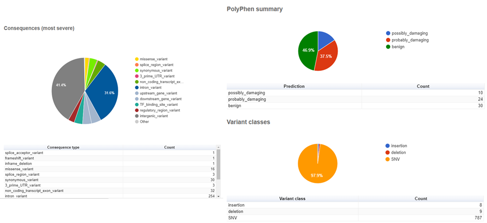
AnnotationVEP.txt and AnnotationVEP.html: outputs of annotation by Ensembl’s VEP. The text file is tab-separated file listing the called variants and their characteristics (more on that later). The HTML file contains a summarized quantification of the variants characteristics.

Open the SRR6784104_AnnotationVEP.txt file into a spreadsheet to make the visualization easier. You will see there is a header with several definitions/abbreviations for the information contained in the file. Scroll down until you found a table-like part.

In this table part, there is several important information that is interesting to check. Some of the columns I like to assess:

#Uploaded_variation: an identifier of each variation;
Location: chromosome and position of the variation;
Allele: particular nucleotide configuration found in determined position in the sample;
Gene: if the variant is located within a gene, its unique RefSeq gene ID (an integer) will be there;
Feature: if the variant is located within a gene, a unique RefSeq accession code of the gene sequence will be there;
Consequence: I found this column weirdly-named, because it reflects more the overall location of the variant than a molecular consequence as the name implies. For example, it will indicate that the variant is a missense_variant, an intron_variant, regulatory_region_variant and so on;
Protein_position, Amino_acids, Codons: if missense or synonym, information about amino acids changes and position on the protein will be in these columns;
Existing_variation: if variation was already previously identified in other samples, the RefSeq (starting with rs) or other identifier will be there. RefSeq-identified variants can be found in NCBI’s dbSNP;
IMPACT: the variant’s impact on phenotype (LOW, MODIFIER, HIGH);
VARIANT_CLASS: the class of the variant. SNV (single nucleotide variation, the same as single nucleotied polymorphism — SNP), insertions and deletions are the most common;
SYMBOL: the official symbol (abbreviation) of the gene name;
BIOTYPE: if the variant is located within a gene, the gene function. For example: protein_coding, lncRNA, miRNA, and so on;
SIFT and PolyPhen: named after the tools that predict whether an amino acid substitution affects protein function and structure of a human protein;
Columns prefixed with AF: contain the allelic frequency of a given variant in some global populations. For example, AFR: African,AMR: Ad Mixed American, EAS: East Asian, SAS: South Asian;
CLIN_SIG: a short sentence stating the clinical significance (if available) of the variant;
PUBMED: a list of PubMed IDs of references citing the variation (if available).

The AnnotationVEP.html file contains a collection of graphical representations of several characteristics of the detected variants. See below some of them. Notice that your results will be different from these figures, since I used a different set of FASTQ files and reference files.

demo results 3

Conclusion of Part 4

In this part I showed:

How to use the FastQ_to_Annotation.sh script;
Summarized the steps performed by the script;
Summarized the principal results output by the script.

Therefore, I finished all the steps I followed to prepare the system for Bioinformatics analysis, gather the necessary files and apply them to obtain annotations from human genome NGS reads samples.

Subscribe to my rss feed or Atom feed to keep updated whenever I post new protocols.

Go back to FASTQ to Annotation (Part 1)

Go back to FASTQ to Annotation (Part 2)

Go back to FASTQ to Annotation (Part 3)