Machine Learning with Python: Supervised Classification of TCGA Prostate Cancer Data (Part 2 - Making a Model)

Posted on Thu 05 November 2020 in Python

Introduction

In a previous post, I showed how to retrieve The Cancer Genome Atlas (TCGA) data from the Cancer Genomics Cloud (CGC) platform. I downloaded gene expression quantification data, created a relational database with PostgreSQL, and created a dataset uniting the raw quantification data for 675 differentially expressed genes identified by edgeR, race, age at diagnosis and tumor size at diagnosis.

In Part 1, I used Python to prepare features datasets to use them to produce a classification model using machine learning tools, especially the scikit-learn module. Check its documentation here.

Here in Part 2, I develop an illustrative model. If it were a serious model, its objective would be to predict if a person is in risk of developing prostate cancer based on personal characteristics and the expression of differentially expressed genes.

The dataset and code presented here are available in my portfolio.

Prepare workspace

As in Part 1, I will import the modules needed to make the model (check the make_model.py script located on src/models):

import pickle
from pathlib import Path

import matplotlib.pyplot as plt
import numpy as np
import pandas as pd
import xgboost
from sklearn.metrics import accuracy_score, precision_score, recall_score, f1_score, roc_auc_score, confusion_matrix, roc_curve, precision_recall_curve
from sklearn.dummy import DummyClassifier
from sklearn.ensemble import RandomForestClassifier
from sklearn.linear_model import LogisticRegression
from sklearn.model_selection import StratifiedKFold, GridSearchCV, KFold, cross_val_score
from sklearn.naive_bayes import GaussianNB
from sklearn.neighbors import KNeighborsClassifier
from sklearn.svm import SVC
from sklearn.tree import DecisionTreeClassifier

Install all non-standard library modules using your Python package manager, usually pip or through anaconda, if you are using a conda environment with Python.

Again, I will set up some constants to use later:

RANDOM_SEED = 42
SPLITS = 10

Set up the file paths:

project_folder = Path().resolve().parent.parent
features_folder = project_folder / "data" / "processed"

Importing features

If you still have the features datasets loaded on memory, the commands below are not necessary. They serve to de-serialize the pickled datasets I saved in Part 1 using pandas‘ read_pickle() method:

X_train = pd.read_pickle(features_folder / "X_train")
X_test = pd.read_pickle(features_folder / "X_test")
y_train = pd.read_pickle(features_folder / "y_train")
y_test = pd.read_pickle(features_folder / "y_test")

Select classification model

The scikit-learn module contains code for several classification models. If you are in doubt, you can select from a list of models using a scoring metric, and the choose the best-performing model. See below a loop command that do just that (hat tip to Matt Harrison):

models = [
DummyClassifier,
LogisticRegression,
DecisionTreeClassifier,
KNeighborsClassifier,
GaussianNB,
SVC,
RandomForestClassifier,
xgboost.XGBClassifier,
]

for model in models:
    cls = model()

    kfold = KFold(n_splits=SPLITS, random_state=RANDOM_SEED)

    s = cross_val_score(cls, X_train, y_train, scoring="f1", cv=kfold)

    print(f"{model.__name__:22}  F1 Score: " f"{s.mean():.3f} STD: {s.std():.2f}")

I will now explain what the loop does. First, I create a list named models with the name of some sklearn models. Note the way their names are written: they are the names of the corresponding sklearn modules.

I then loop this list creating a classifier cls object by calling each model. Then, I create a K-Folds cross-validator. In other words, I randomly split the training dataset into K datasets (folds). Each fold is then used once as a validation while the K - 1 remaining folds form the training set. The n_splits argument indicates K, which I set up using the SPLITS constant (currently 10, so K=10 folds). Setting a integer (RANDOM_SEED constant) into the random_state argument ensures that the splitting outputs can be reproduced.

Next, I calculate the F1 Score by comparing the predictions with their actual labels (y_train series). As the text in the linked page states, “it is calculated from the precision and recall of the test, where the precision is the number of correctly identified positive results divided by the number of all positive results, including those not identified correctly, and the recall is the number of correctly identified positive results divided by the number of all samples that should have been identified as positive”. Recall is also named true positive rate (TPR) and sensitivity. The F1 Score is the harmonic mean of the precision and recall. This calculation is performed by cross_val_score() method from sklearn.model_selection module for each comparison among the folds. Then, the final result is an average of all measurements, which is stored at the s object. Finally, the loop ends printing the mean F1 Score and its standard deviation (STD).

Why I chose the F1 Score? Because there is class imbalance in the data: there is much more control than cases in the dataset. Thus, scores such as accuracy and precision may be misleading when considered alone. The Wikipedia article about sensitivity and specificity is a great summary of these concepts.

After a while, the output will be printed to your console. It will be something like this:

DummyClassifier         F1 Score: 0.248 STD: 0.16
LogisticRegression      F1 Score: 0.578 STD: 0.28
DecisionTreeClassifier  F1 Score: 0.291 STD: 0.19
KNeighborsClassifier    F1 Score: 0.069 STD: 0.14
GaussianNB              F1 Score: 0.399 STD: 0.27
SVC                     F1 Score: 0.165 STD: 0.31
RandomForestClassifier  F1 Score: 0.337 STD: 0.26
XGBClassifier           F1 Score: 0.370 STD: 0.34

The dataset folds will be identical, but you may have different values in some of these models due to stochasticity during calculation. Nevertheless, the values should be close enough. It seems that LogisticRegression had the best performance among the models, with a rounded up F1 Score = 0.58. So I will continue with this model and try to improve the F1 Score by optimizing (tuning) the model.

Model optimization

I will now setup the model and produce a grid of hyperparameters. A hyperparameter is a parameter of the model whose value affects the learning/classification process. A grid is therefore a collection of some of those hyperparameters that I will give to the model so it can choose the best candidates. I now set up the model:

estimator = LogisticRegression()

And this is the grid:

grid = {"penalty":["l1", "l2", "elasticnet","none"],
"dual":[False, True],
"C":np.logspace(-3,3,7)
}

Note that each model has different hyperparameters; those above are logistic regression-exclusive. Check the sklearn.linear_model.LogisticRegression module documentation to know more about these hyperparameters.

Now, I pass the model (assigned to estimator object) to the GridSearchCV function so that it returns the optimal parameters during fitting to the train data with 10-fold cross-validation:

logreg_cv=GridSearchCV(estimator,grid,cv=SPLITS)
logreg_cv.fit(X_train,y_train)

Let’s see a summary of the candidates:

print("tuned hyperparameters :(best parameters) ",logreg_cv.best_params_)

The output will be:

tuned hyperparameters :(best parameters)  {'C': 100.0, 'dual': False, 'penalty': 'l2'}

Now I pass the best parameters as keywords to the optimized model, which I will assign to logreg object, and then fit the training data once again:

logreg = LogisticRegression(**logreg_cv.best_params_)
logreg.fit(X_train, y_train)

With the fitted model, I can now generate predictions with the test dataset:

predictions = logreg.predict(X_test)
predicted_proba = logreg.predict_proba(X_test)

Evaluate model performance

Let’s compare the predict labels with actual classification using a confusion matrix:

conf_matrix = pd.DataFrame(data=confusion_matrix(y_test, predictions).T,index=["Prediction: controls", "Prediction: cases"], columns=["Actual: controls", "Actual: cases"])

print(conf_matrix)

The output will be:

#                  Actual: controls  Actual: cases
Prediction: controls                47             11
Prediction: cases                    8              5

Now remember the labels summary I got in Part 1:

Training Set has 38 Positive Labels (cases) and 127 Negative Labels (controls)
Test Set has 16 Positive Labels (cases) and 55 Negative Labels (controls)

Thus, the model erroneously classified 11 (of 16) cases as controls (false negatives) and correctly classified 5 (of 16) cases as cases (true positives). If this model were to be used in a real world scenario, this would be a problem, because the model would miss people at risk of disease progression.

Imagine that detecting prostate cancer disease progression risk will trigger further analysis (gather second opinion, ask the patients more examinations etc.) whereas if you don’t detect this risk, the patient would be sent home with the disease actively progressing. In this situation, therefore, I would prefer false positives (type I error) over false negatives (type II error).

Please note that there is not a single response for every classification problem; the researcher must evaluate the consequences of the errors and make a decision, since reducing one type of error means increasing the other type of error. In every situation, one type of error is more preferable than the other one — it is always a trade-off.

But why the model incorrectly classified some patients? One of the factors is because logistic regression models calculate probabilities to make these predictions. If the predicted probability from a sample is >= 0.50, it labels the sample as case, otherwise, it labels as a control. I can change this probability cutoff to try to reduce the number of false negatives, especially since there is class imbalance in the dataset.

Using the data in this confusion matrix, I can calculate and print some metrics:

print(f"Accuracy: {accuracy_score(y_test, predictions):.3f}")
print(f"Precision: {precision_score(y_test, predictions):.3f}")
print(f"Recall: {recall_score(y_test, predictions):.3f}")
print(f"F1 Score: {f1_score(y_test, predictions):.3f}")

The output:

Accuracy: 0.732
Precision: 0.385
Recall: 0.312
F1 Score: 0.345

I can also print a receiver operating characteristic (ROC) curve. As stated in the Wikipedia article, it “illustrates the diagnostic ability of a binary classifier system as its discrimination threshold is varied”. The area under the ROC curve (AUC) summarizes the predictive power of the model.

false_pos_rate, true_pos_rate, proba = roc_curve(y_test, predicted_proba[:, -1])
plt.figure()
plt.plot([0,1], [0,1], linestyle="--") # plot random curve
plt.plot(false_pos_rate, true_pos_rate, marker=".", label=f"AUC = {roc_auc_score(y_test, predicted_proba[:, -1]):.2f}")
plt.title("ROC Curve")
plt.ylabel("True Positive Rate")
plt.xlabel("False Positive Rate")
plt.legend(loc="lower right")

The output:

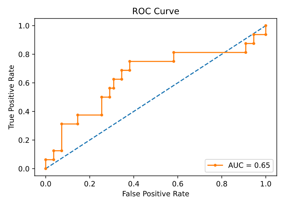
ROC curve from logistic regression model classifying TCGA prostate cancer dataset

The AUC is equal to the probability that the model will rank a randomly chosen positive instance higher than a randomly chosen negative one. It ranges from 0 to 1 (perfect classifier). A random, thus useless, classifier, has a AUC = 0.5. Since the AUC of my model is about 0.65, means that it has some predictive power, although not perfect. I cannot improve the AUC, but I can change the classification probability threshold (as I mentioned above) to try to better utilize the potential of the model.

Change classification threshold

Looking at the metrics I printed above, I can see the model has fairly low sensitivity (recall) as well as low F1 score. Since there is class imbalance, I will change the classification threshold based on F1 score.

I now calculate the range of F1 scores with several classification thresholds:

precision, recall, thresholds = precision_recall_curve(y_test, predicted_proba[:, -1])

f1_scores = 2 * recall * precision / (recall + precision)

The precision_recall_curve() function will select a classification threshold (thresholds object), label the samples according to their predicted probabilities given by the model (predicted_proba[:, -1]) and compare with the actual labels (y_test), calculating the precision and recall (precision and recall objects).

All three objects are NumPy arrays. Thus, I can obtain the probability cutoff value associated with maximum F1 score, and create a list of prediction labels and assign to f1_predictions object using a list comprehension with a if else statement:

optimal_proba_cutoff = thresholds[np.argmax(f1_scores)]

f1_predictions = [1 if i >= optimal_proba_cutoff else 0 for i in predicted_proba[:, -1]]

Let’s examine the confusion matrix using this new cutoff:

conf_matrix_th = pd.DataFrame(data=confusion_matrix(y_test, f1_predictions).T, index=["Prediction: controls", "Prediction: cases"], columns=["Actual: controls", "Actual: cases"])
print(conf_matrix_th)

The output:

#                  Actual: controls  Actual: cases
Prediction: controls                34              4
Prediction: cases                   21             12

I can see that I reduced the number of false negatives at the cost of having more false positives, as discussed above. Now the model erroneously classified just 4 cases as controls, compared to 11 before thresholding. Let’s calculate the model’s metrics again:

print(f"Accuracy Before: {accuracy_score(y_test, predictions):.3f} --> Now: {accuracy_score(y_test, f1_predictions):.3f}")
print(f"Precision Before: {precision_score(y_test, predictions):.3f} --> Now: {precision_score(y_test, f1_predictions):.3f}")
print(f"Recall Before: {recall_score(y_test, predictions):.3f} --> Now: {recall_score(y_test, f1_predictions):.3f}")
print(f"F1 Score Before: {f1_score(y_test, predictions):.3f} --> Now: {f1_score(y_test, f1_predictions):.3f}")

The output:

Accuracy Before: 0.732 --> Now: 0.648
Precision Before: 0.385 --> Now: 0.364
Recall Before: 0.312 --> Now: 0.750
F1 Score Before: 0.345 --> Now: 0.490

I see that the sensitivity (recall) improved greatly, with a consequential F1 score improvement. With the current data, this is the maximum improvement I can achieve. If this model would to be used in a real world scenario, I would have to gather more information to try to further improve the classification power of the model, always assessing the optimal probability cutoff to account for class imbalance.

Save (Serialize) model

I can save the model to disk as a pickled object to use in the future or share with someone. Remember that the same modules must be installed and loaded in the system that will receive the pickled model so it can be unpickled and work correctly. See below the commands to save the model and the chosen probability cutoff for classification:

pickle.dump(logreg, open(project_folder / "models" / "logreg", "wb"))
pickle.dump(optimal_proba_cutoff, open(project_folder / "models" / "logreg", "wb"))

Note: pickled objects are Python-specific only — non-Python programs may not be able to reconstruct pickled Python objects. WARNING: never, NEVER, unpickle data you do not trust. As it says in the Python documentation: “It is possible to construct malicious pickle data which will execute arbitrary code during unpickling”.

Below is a schematics of my working directory. Check it on my porfolio:

.
├── data
│   ├── interim
│   │   └── prostate_cancer_dataset.csv
│   └── processed
│       ├── X_train
│       ├── X_test
│       ├── y_train
│       └── y_test
├── models
│   ├── logreg
│   └── optimal_proba_cutoff
└── src
    ├── features
    │   └── make_features.py
    └── models
        └── make_model.py